How to do linear regression in R

Linear regression. It’s a technique that almost every data scientist needs to know.

Although machine learning and artificial intelligence have developed much more sophisticated techniques, linear regression is still a tried-and-true staple of data science.

In this blog post, I’ll show you how to do linear regression in R.

Before I actually show you the nuts and bolts of linear regression in R though, let’s quickly review the basic concepts of linear regression.

A quick review of linear regression concepts

Linear regression is fairly straight forward.

Let’s start with the simplest case of simple linear regression. We have two variables in a dataset, X and Y.

We want to predict Y. Y is the “target” variable.

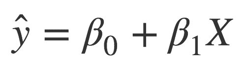
We make the assumption that we can predict Y by using X. Specifically, we assume that there is a linear relationship between Y and X as follows:

If you haven’t seen this before, don’t let the symbols intimidate you. If you’ve taken highschool algebra, you probably remember the equation for a line, , where is the slope and is the intercept.

The equation for linear regression is essentially the same, except the symbols are a little different:

Basically, this is just the equation for a line. is the intercept and is the slope.

In linear regression, we’re making predictions by drawing straight lines

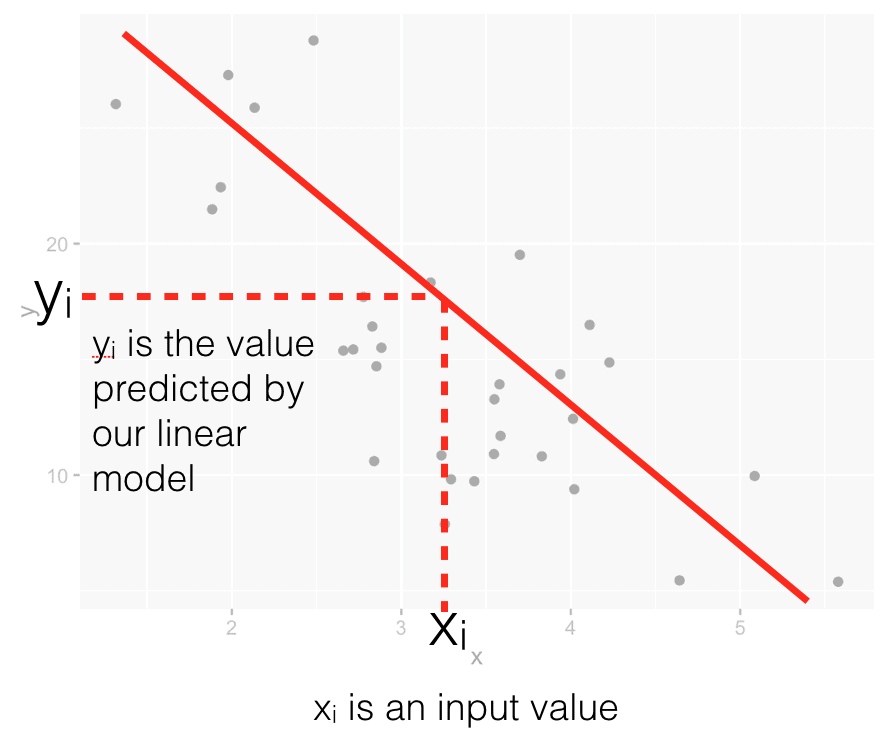
To clarify this a little more, let’s look at simple linear regression visually.

Essentially, when we use linear regression, we’re making predictions by drawing straight lines through a dataset.

To do this, we use an existing dataset as “training examples.” When we draw a line through those datapoints, we’re “training” a linear regression model. By the way, this input dataset is typically called a training dataset in machine learning and model building.

When we draw such a line through the training dataset, we’ll essentially have a little model of the form by using the formula . Remember: a line that we draw through the data will have an equation associated with it.

This equation is effectively a model that we can use that linear model to make predictions.

For example, let’s say that after building the model (i.e., drawing a line through the training data), we have a new input value, . To make a prediction with our simple linear regression model, we’re just need to use that datapoint as an input to our linear equation. If you know the value, you can compute the predicted output value, by using the formula .

We can visualize that as follows:

This should give you a good conceptual foundation of how linear regression works.

You:

1. Obtain a training dataset
2. Draw the “best fit” line through the training data
3. Use the equation for the line as a “model” to make predictions

I’m simplifying a little, but that’s essentially it.

The critical step though is drawing the “best” line through your training data.

Linear regression is about finding the “best fit” line

So the hard part in all of this is drawing the “best” straight line through the original training dataset. A little more specifically, this all comes down to computing the “best” coefficient values: and … the intercept and slope.

Mathematically it’s not terribly complicated, but I’m not going to explain the nuts and bolts of how it’s done.

Instead, I’ll show you now how to use R to perform linear regression. By using R (or another modern data science programming language), we can let software do the heavy lifting; we can use software tools to compute the best fit line.

With that in mind, let’s talk about the syntax for how to do linear regression in R.

How to do linear regression in R

There are several ways to do linear regression in R.

Nevertheless, I’m going to show you how to do linear regression with base R.

I actually think that performing linear regression with R’s caret package is better, but using the lm() function from base R is still very common. Because the base R methodology is so common, I’m going to focus on the base R method in this post.

How to do linear regression with base R

Performing a linear regression with base R is fairly straightforward. You need an input dataset (a dataframe). That input dataset needs to have a “target” variable and at least one predictor variable.

Then, you can use the lm() function to build a model. lm() will compute the best fit values for the intercept and slope – and . It will effectively find the “best fit” line through the data … all you need to know is the right syntax.

Syntax for linear regression in R using lm()

The syntax for doing a linear regression in R using the lm() function is very straightforward.

First, let’s talk about the dataset. You tell lm() the training data by using the data = parameter.

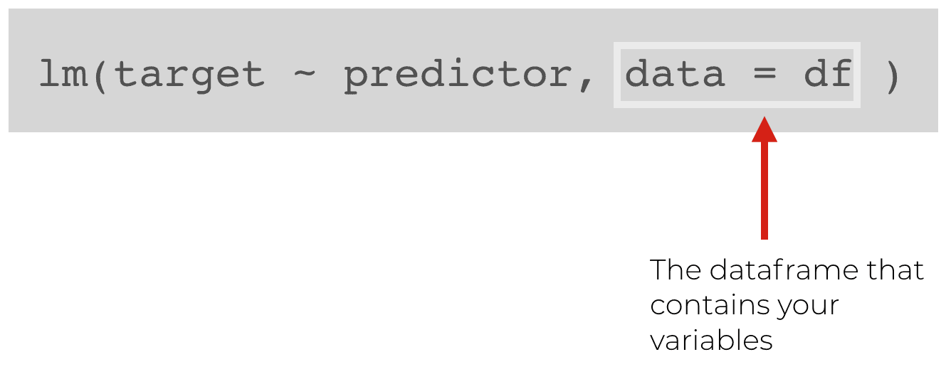
So when we use the lm() function, we indicate the dataframe using the data = parameter.

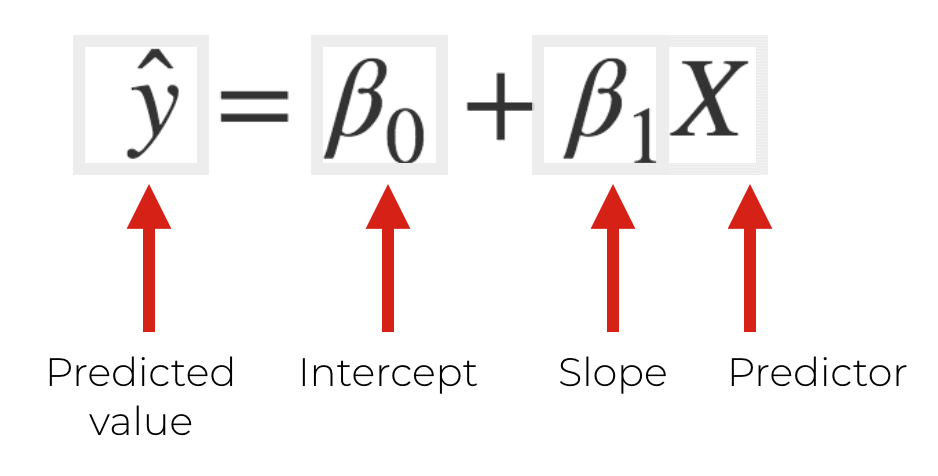
We also need to provide a “formula” that specifies the target we are trying to predict as well as the input(s) we will use to predict that target:

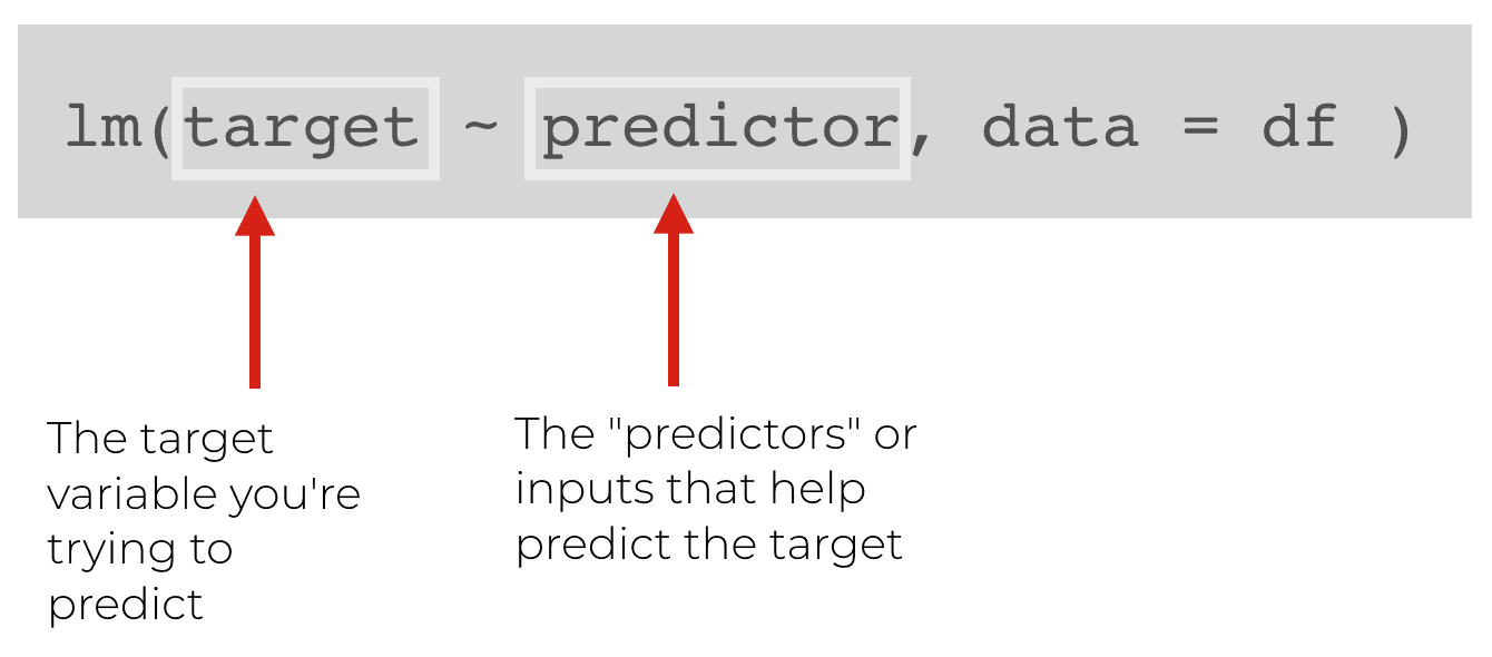
Notice the syntax: target ~ predictor. This syntax is basically telling the lm() function what our “target” variable is (the variable we want to predict) and what our “predictor” variable is (the x variable that we’re using as an input to for the prediction). In other words, we will predict the “target” as a function of the “predictor” variable.

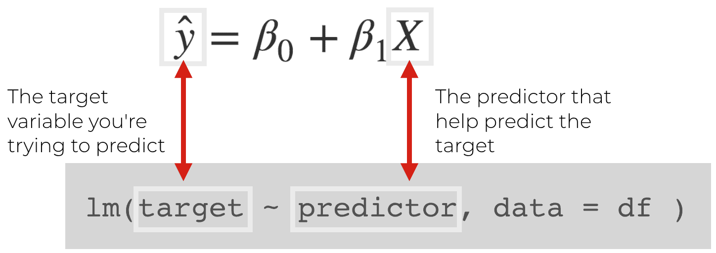
Keep in mind that this aligns with the equation that we talked about earlier. We’re trying to predict a “target” (which is typically denoted as ) on the basis of a predictor, X.

When you use lm(), it’s going to take your training dataset (the input dataframe) and it will find the best fit line.

More specifically, the lm() function will compute the slope and intercept values – and – that will fit the training dataset best. You give it the predictors and the targets, and lm() will find the remaining parts of the prediction equation: and .

Example: linear regression in R with lm()

This might still seem a little abstract, so let’s take a look at a concrete example.

Create data

First, we’ll just create a simple dataset.

This is pretty straightforward … we’re just creating random numbers for x. The y value is designed to be equal to x, plus some random, normally distributed noise.

Keep in mind, this is a bit of a toy example. On the other hand, it’s good to use toy examples when you’re still trying to master syntax and foundational concepts. (When you practice, you should simplify as much as possible.)

#--------------
# LOAD PACKAGES
#--------------
library(tidyverse)


#------------------------
# CREATE TRAINING DATASET
#------------------------

set.seed(52)
df <- tibble(x = runif(n = 70, min = 0, max = 100)
             , y = x + rnorm(70, mean = 0, sd = 25)
)


# INSPECT
df %>% glimpse()

Visualize training data

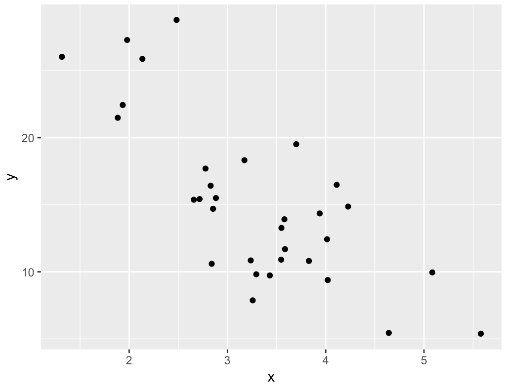
And let’s make a quick scatterplot of the data:

#----------------------------
# VISUALIZE THE TRAINING DATA
#----------------------------
ggplot(data = df, aes(x = x, y = y)) +
  geom_point()

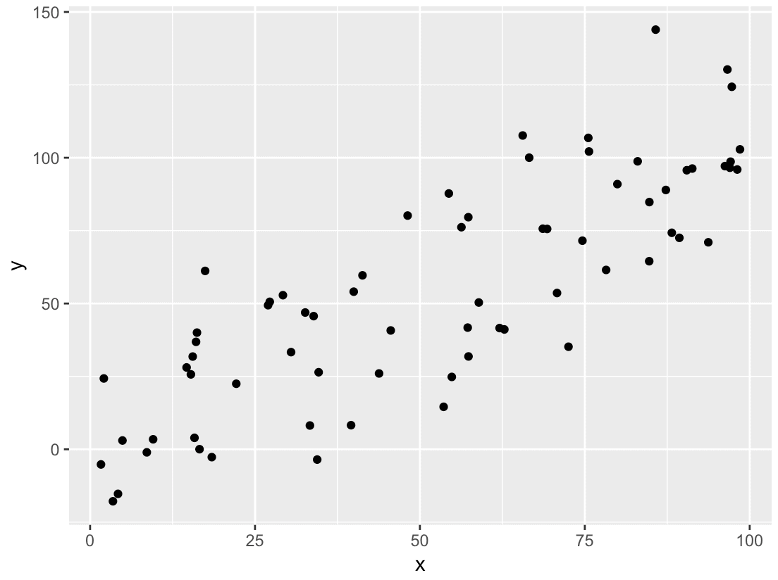
It’s pretty clear that there’s a linear relationship between x and y. Now, let’s use lm() to identify that relationship.

Build model

Here, we’ll let’s create a model using the lm() function.

#===================
# BUILD LINEAR MODEL
#===================

model_linear1 <- lm(y ~ x, data = df)

Get a summary report of the model

We can also get a printout of the characteristics of the model.

To get this, just use the summary() function on the model object:

#=====================================
# RETRIEVE SUMMARY STATISTICS OF MODEL
#=====================================
summary(model_linear1)

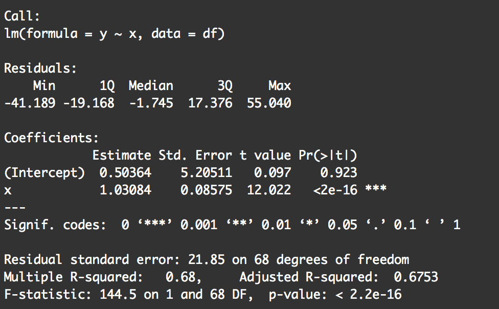
Notice that this summary tells us a few things:

1. The coefficients
2. Information about the residuals (which we haven't really discussed in this blog post
3. Some "fit" statistics like "residual standard error" and "R squared"

Visualize the model

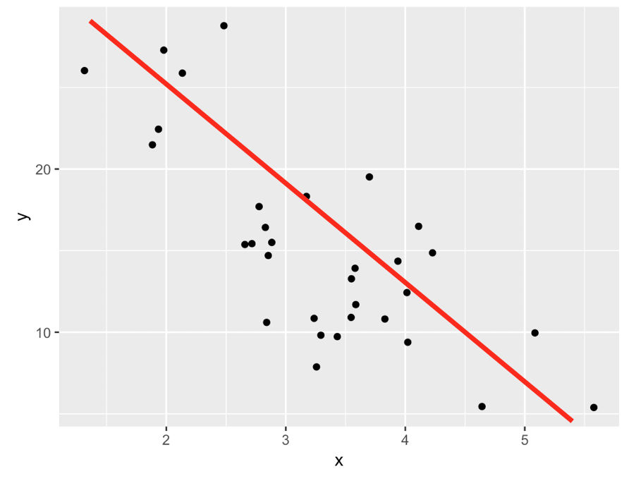
Now that we have the model, we can visualize it by overlaying it over the original training data.

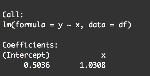
To do this, we'll extract the slope and intercept from the model object and then plot the line over the training data using ggplot2.

#====================
# VISUALIZE THE MODEL
#====================

model_intercept <- coef(model_linear1)[1]
model_slope <- coef(model_linear1)[2]


#-----
# PLOT
#-----

ggplot(data = df, aes(x = x, y = y)) +
  geom_point() +
  geom_abline(intercept = model_intercept, slope = model_slope, color = 'red')

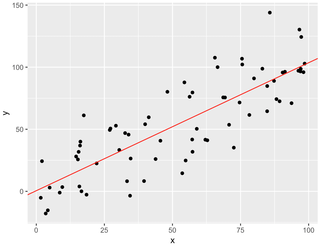
As you look at this, remember what we're actually doing here.

We took a training dataset and used lm() to compute the best fit line through those training data points. Ultimately, this yields a slope and intercept that enable us to draw a line of the form . That line is a model that we can use to make predictions.

Linear regression is an important techniques

As I said at the beginning of the blog post, linear regression is still an important technique. There are many techniques that are sexier and more powerful for specific applications, but linear regression is still an excellent tool to solve many problems.

Moreover, many advanced machine learning techniques are extensions of linear regression.

"Many fancy statistical learning approaches can be seen as extensions or generalizations of linear regression."
– An Introduction to Statistical Learning

Learning linear regression will also give you a basic foundation that you can build on if you want to move on to more advanced machine learning techniques. Many machine learning concepts have roots in linear regression.

Having said that, make sure you study and practice linear regression.

Leave your questions in the comments below

What questions do you still have about linear regression and linear regression in R?

Leave your questions and challenges in the comments below ...