In this tutorial, I’ll explain how to use the np.random.randn function (AKA, Numpy random randn).
The tutorial is divided up into several different sections, including a quick overview of what the function does, an explanation of the syntax, and a section that shows step-by-step examples.
You can click on any of the following links and it will take you to the appropriate section in the tutorial.
Table of Contents:
- Introduction to Numpy Random randn
- The syntax of np.random.randn
- Examples of np.random.randn
- np.random.randn FAQ
Introduction to Numpy Random randn
Let’s start off with a quick introduction to the Numpy random randn function.
Numpy Random Randn Creates Numpy Arrays
As you probably know, the Numpy random randn function is a function from the Numpy package.
Numpy is a library for the Python programming language for working with numerical data.
As such, the functions from Numpy all deal with either creating Numpy arrays or manipulating Numpy arrays.
Numpy random randn does the former; it creates Numpy arrays (with one simple exception, which we will discuss in example 1.
Numpy random randn generates normally distributed numbers
Numpy random randn creates new Numpy arrays, but the numbers returned have a very specific structure: Numpy random randn returns numbers that are generated randomly from the normal distribution.
Remember that the normal distribution is a continuous probability distribution that has the following probability density function:
(1) 
Where  is the mean and
  is the standard deviation.
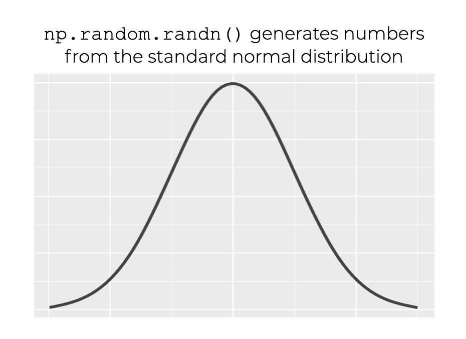
Specifically, np.random.randn generates numbers from the standard normal distribution.
The standard normal distribution is a normal distribution that has a mean of 0 and a standard deviation of 1.
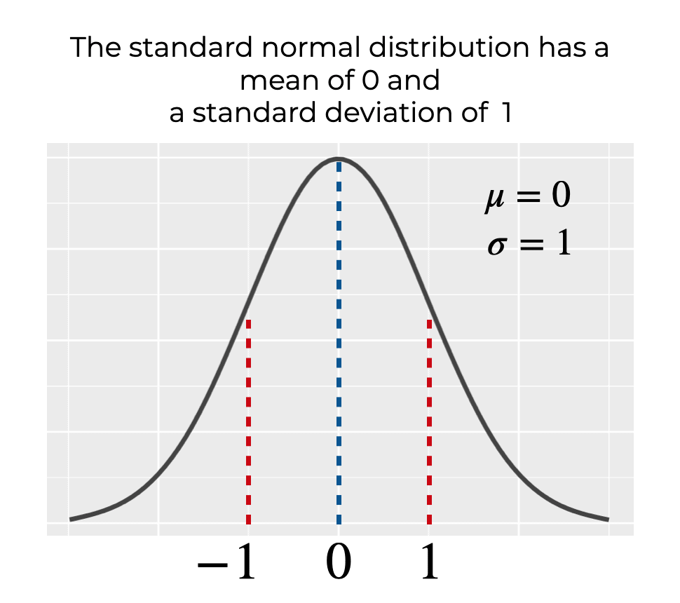
So when we set  and
and  for the standard normal distribution, equation 1 simplifies to the following:
(2) 
Essentially, Numpy random randn generates normally distributed numbers from a normal distribution that has a mean of 0 and a standard deviation of 1.
The syntax of np.random.randn
So now that you know a little about what np.random.randn does, let’s discuss the syntax.
A quick note
One quick note before we look at the syntax.
Whenever we import a Python package in our code, we have the option to import with a particular alias.
How exactly we import a module will slightly change how we call the function.
Here in our code, we’ll import Numpy with the alias ‘np‘ using the following code:
import numpy as np
This is the common convention among Python users.
Because of this import style, we’ll use the prefix ‘np‘ when we call the function.
np.random.randn syntax
Ok, now let’s take a look at the syntax.
When we call the function, assuming that we’ve imported Numpy as discussed above, we can call the function as np.random.randn().
Then, inside the parenthesis, there are a few parameters that we can use.
Let’s take a look at those.
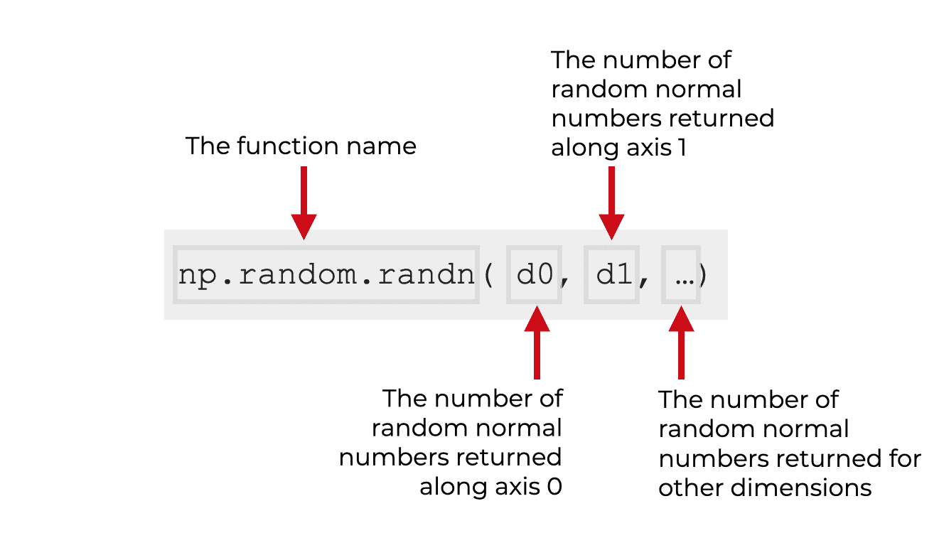
The parameters of np.random.randn
Numpy random randn is actually fairly simple in terms of parameters.
First of all, we can call the function without any parameters.
However, if we do choose to use parameters, we simply provide integer arguments to the parameters that we can call d0, d2, 
dn.
Let’s take a closer look.
d0 (optional)
If we decide to use the d0 parameter, we simply provide an integer as the input.
When we do this, that becomes the number of normally distributed values that np.random.randn will generate along axis 0.
(Remember: axes are like directions along a Numpy array. If you’re confused about Numpy array axes, you should read our tutorial about Numpy axes.)
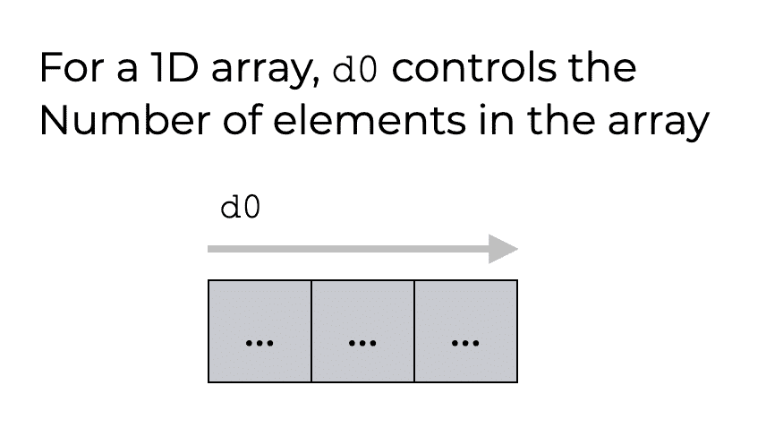
So if we use the code np.random.randn(3), Numpy will generate a new Numpy array with three normally distributed values. You’ll see an example of this in the examples section.
d1 (optional)
The d1 parameter does something very similar to d0.
Remember, d0 specifies the Number of values in the axis 0 direction.
Similarly, d1 specifies the Number of values in the axis 1 direction.
Keep in mind that we can only use d1 if we’re already using d0.
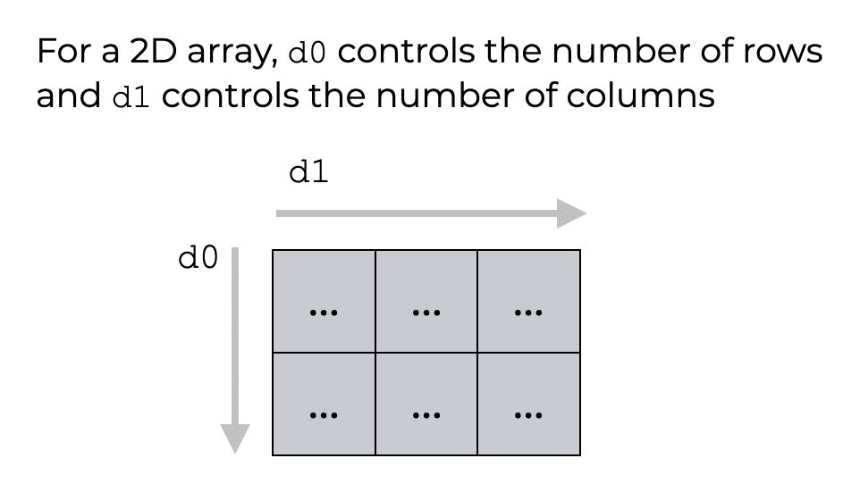
So when we use d0 and d1 (and no additional parameters), we’re essentially telling Numpy to create a 2-dimensional Numpy array, where the number of rows are specified by d0 (axis 0), and the number of columns are specified by d1.
If you’re really a Numpy beginner, this might seem confusing. For a 2D array, d0 controls the rows, but for a 1D array, d0 seems to control the columns, right?
No.
d0 always controls the number of elements in the axis 0 direction. However, the axis 0 direction appears horizontal for 1D arrays, but appears vertical for 2D arrays.
If you’re confused about this, you really, really need to learn more about Numpy axes, so please read our Numpy axis tutorial.
dn (optional)
Beyond d0 and d1, there are actually more parameters for np.random.randn().
All of these additional parameters control the number of elements along a particular axis, for the output array.
So d2 controls the number of elements along axis 2. d3 controls the number of elements along axis 3, and so on.
These parameters are completely optional. You’re only going to use them if you need to create Numpy arrays with a larger number of dimensions (i.e., beyond 1D or 2D arrays).
The Output of np.random.randn
The output of Numpy random randn depends on how you call the function.
If you use the parameters (i.e., d0, d1, dn), the output will be a Numpy array with dimensions (d0, d1, ..., dn). All of the numbers in the ouput array will be drawn from the standard normal distribution, as described by equation 2.
However, if you call the function without any parameters – i.e., np.random.randn() with nothing inside the parenthesis – then the function will return a single floating point number drawn from the standard normal distribution.
Examples of How to Use np.random.randn
Ok. Let’s take a look at some examples. The syntax and parameters will make a lot more sense once you can play with some code and see how it works..
Examples:
- Generate a single number with np.random.randn
- Create a 1D Numpy array with Numpy Random Randn
- Create a 2D Numpy array with Numpy Random Randn
You can click on any of the above links, and they will take you to the appropriate example.
Run this code first
One quick note …
As explained in the section about syntax, how we write the syntax depends partially on how we’ve imported Numpy.
We’re going to import Numpy with the alias ‘np‘, which you can do with the following code:
import numpy as np
This is the common convention among Python data scientists, and we’ll be using it going forward.
EXAMPLE 1: Generate a single number with np.random.randn
First, let’s just generate a single random normal number np.random.randn.
Here, we’re going to call the function without any arguments to the parameters.
np.random.seed(0)
np.random.randn()
OUT:
1.764052345967664
Explanation
When we use np.random.randn() like this, without any inputs, it simply returns a number that’s drawn randomly from the standard normal distribution.
Keep in mind that in this example, we’ve used the Numpy random seed function as well. By setting np.random.seed(0), we’ll get the same number every single time we run np.random.randn(). If we use a different seed (besides 0), we’ll get a different number. And if we don’t use np.random.seed at all, we’ll get a different normally distributed number every time. Essentially, we use Numpy random seed when we want the output of our code to be reproducable.
(If you’re confused about this, you need to read our guide to Numpy random seed.)
EXAMPLE 2: Create a 1D Numpy array with Numpy Random Randn
Next, we’ll create a 1-dimensional array with Numpy random randn.
To do this, we’re going to call np.random.randn() with a single argument (i.e., an input to the function).
np.random.seed(0)
np.random.randn(3)
OUT:
array([1.76405235, 0.40015721, 0.97873798])
Explanation
Here, we used the input value 3 as the argument to the function.
This value is being passed to the d0 parameter, which controls the number of elements along axis 0.
Here, since we’re only passing a value to d0 (and not any other parameters), this creates a 1-dimensional array with 3 values.
(Note: we’re using Numpy random seed function for reproducibility. See example 1 for an explanation.)
EXAMPLE 3: Generate a 2D Numpy array with Numpy Random Randn
Finally, let’s create a 2-dimensional numpy array.
To do this, we’ll pass two integer input values to the function.
np.random.seed(0)
np.random.randn(2,3)
OUT:
array([[ 1.76405235,  0.40015721,  0.97873798],
       [ 2.2408932 ,  1.86755799, -0.97727788]])
Explanation
Notice the shape of the output.
The output array has 2 rows and 3 columns.
That’s because we called the function as np.random.randn(2,3).
The first number, 2, controls the number of elements along axis 0. Remember, for a 2D array, axis 0 is the rows.
The second number, 3, controls the number of elements along axis 1. Remember, for a 2D array, axis 1 is the columns.
If you’re confused about this, go back and re-read the syntax section, which explains the function parameters.
(Note: again, we’re using Numpy random seed function for reproducibility. See example 1 for an explanation.)
Frequently asked questions about Numpy Random Randn
Now that you’ve seen some examples, let’s quickly discuss one common question about numpy random randn.
Question 1: What’s the difference between np.random.randn and np.random.normal?
These two functions, np.random.randn and np.random.normal, are very similar.
Both functions produce data that’s drawn from a normal distribution.
The major difference is that np.random.randn only draws numbers from the standard normal distribution, which has and .
However, np.random.normal can essentially draw numbers from a normal distribution with any mean and any standard deviation.
Another way of saying this is that np.random.normal allows us to manually set the mean and standard deviation, but for np.random.randn, the mean and standard deviation are strictly set.
So for example, if we manually set and for np.random.normal, they will create the same output (assuming that we set the same shape).
Here’s an example.
Run the code for both of these.
np.random.seed(0)
np.random.randn(2,3)
np.random.seed(0)
np.random.normal(size = (2,3), loc = 0, scale = 1)
You’ll find that they produce the same output.
OUT:
array([[ 1.76405235,  0.40015721,  0.97873798],
       [ 2.2408932 ,  1.86755799, -0.97727788]])
Again, numpy.random.randn and numpy.random.normal both produce numbers drawn from the normal distribution.
The difference is that numpy.random.normal gives you more control over the mean and standard deviation.
Ultimately, numpy.random.randn is like a special case of numpy.random.normal with loc = 0 and scale = 1.
Leave your other questions in the comments below
Do you have other questions about the Numpy random randn function?
If so, just leave your question in the comments section at the bottom of the page.
Join our course to learn more about Numpy
The examples here about Numpy floor are pretty simple and easy to understand.
But other parts of Numpy can be a lot more complicated.
If you’re serious about learning Numpy (and serious about data science in Python), you should consider joining our premium course called Numpy Mastery.
Numpy Mastery will teach you everything you need to know about Numpy, including:
- How to create Numpy arrays
- How to use the Numpy random functions
- What the “Numpy random seed” function does
- How to reshape, split, and combine your Numpy arrays
- How to perform mathematical operations on Numpy arrays
- and more …
Moreover, it will help you completely master the syntax within a few weeks. We’ll show you a practice system that will enable you to memorize all of the Numpy syntax you learn. If you have trouble remembering Numpy syntax, this is the course you’ve been looking for.
Find out more here:
The second number, 3, controls the number of elements along axis 1. Remember, for a 2D array, axis 0 is the columns.
In the above, I think that ((axis 0 is the columns)) is wrong and must be:
((axis 0 is the rows)). Because of, in 2D-array axis-0 controls the rows.
Good catch. That was a typo.
It should say “The second number, 3, controls the number of elements along axis 1. Remember, for a 2D array, axis 1 is the columns.”