A Quick Introduction to the Python Pandas Package

This tutorial will explain the Python Pandas package. It will explain what Pandas is, how we use it, and why it’s important.

Here’s a quick overview of the different sections of the article.

You can click on any of these links, and it will take you to the appropriate section if you need something specific:

Table of Contents:

• Introduction to Pandas
• Introduction to Dataframes
• Pandas Data Manipulation Methods
• How to “Chain” Pandas Methods Together

A Quick Introduction to Pandas

First off, let’s just quickly review what Pandas is.

Pandas is a data science toolkit for doing data wrangling in Python.

You’re probably aware that data wrangling (AKA, data manipulation) is extremely important in data science. In fact, there’s a saying in data science that “80% of your work in data science will be data wrangling.”

Although the reality is a bit more nuanced, that saying is mostly true.

So if you’re doing data science in Python, you need a toolkit for “wrangling” your data. That’s what Pandas provides.

Pandas gives you tools to modify, filter, transpose, reshape, and otherwise clean up your Python data.

But it’s mostly set up to work with data in a particular data structure … the Pandas dataframe.

That being the case, let’s quickly review what dataframes are.

A Quick Introduction to Pandas Dataframes

The Pandas dataframe is a special data structure in Python.

Dataframes store data in a row-and-column format that’s very similar to an Excel spreadsheet.

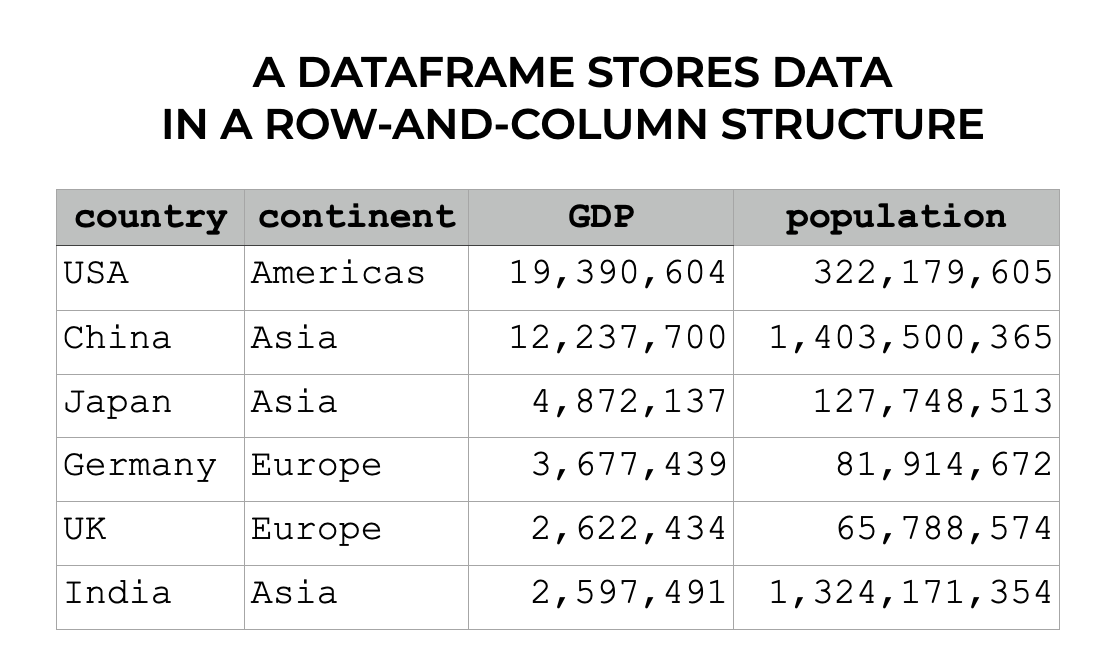
So dataframes have rows and columns. Each column has a label (i.e., the column name), and rows can also have a special label that “index,” which is like a label for a row.

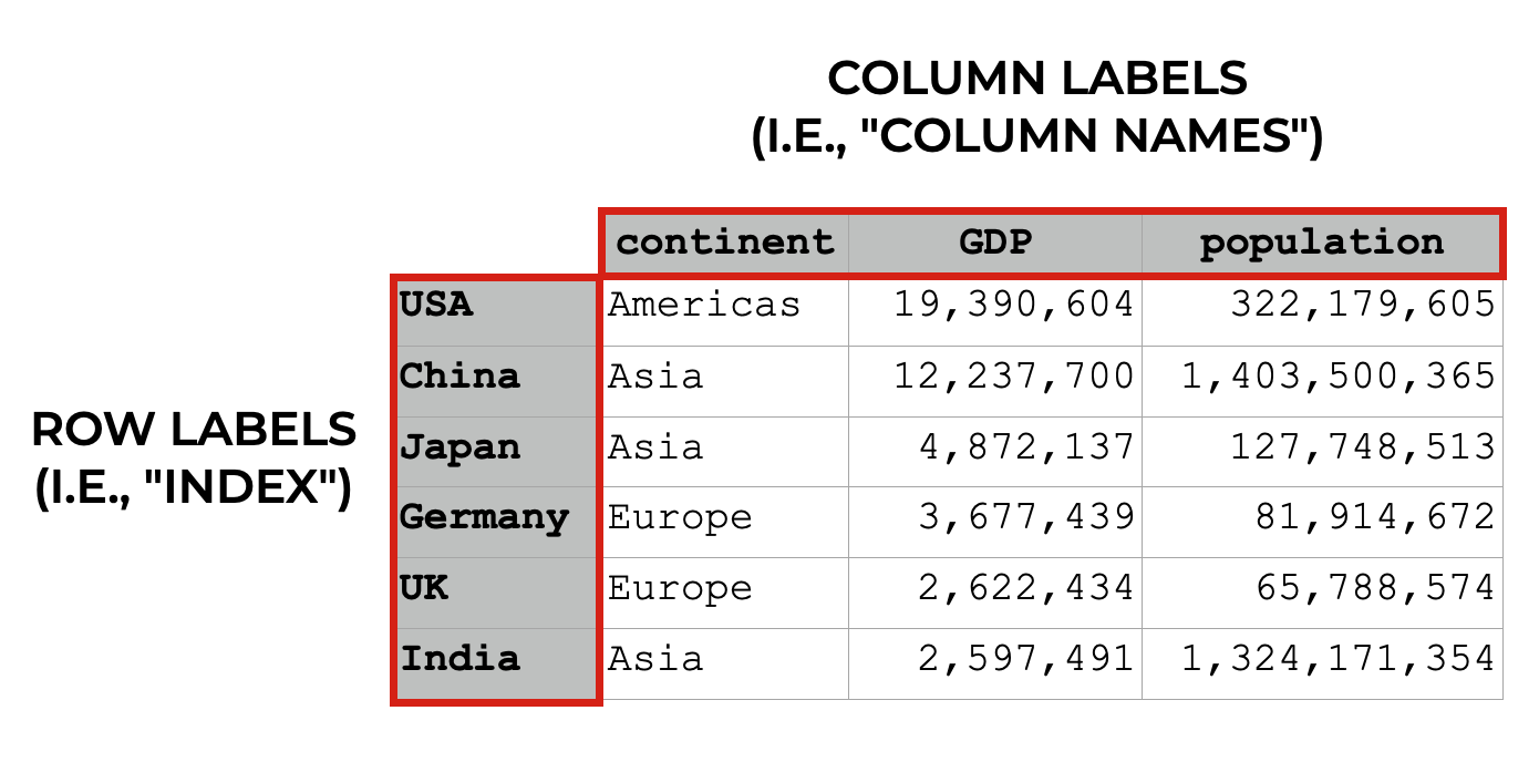
Keep in mind that dataframe indexes are a little complicated, so to understand them better, check out our tutorial on the Pandas dataframe indexes or our tutorial on the Pandas set index method.

Different columns can have different types of data

Importantly, different columns can have different types of data.

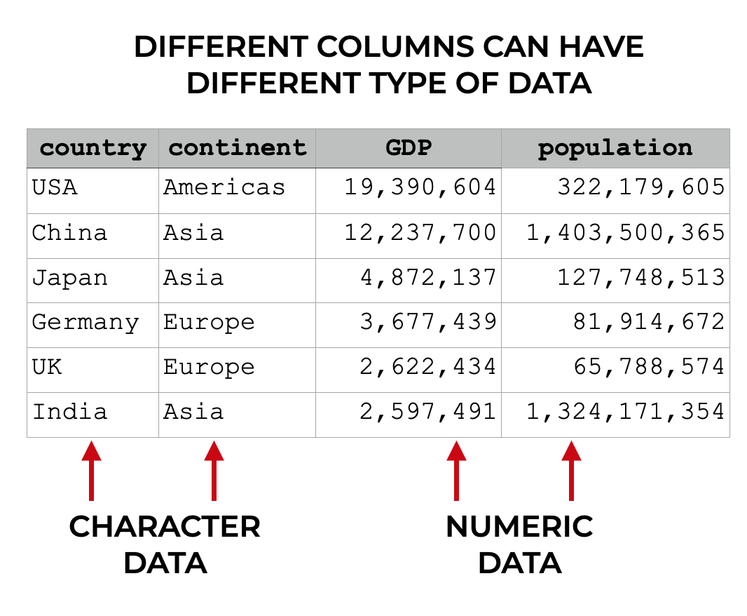
So one column might have string data (i.e., character data). But another column might have int data (i.e., numeric integer data). Different columns can contain different datatypes.

Having said that, all of the data within a column needs to be of the same type. So a for a column that has string data, all of the data will be string data. For a column that has float data, all of the data will be floating point numbers.

Sometimes, We Need to Clean or Reshape Our Data

In the examples that I’ve just shown you in the previous sections, the dataframes were pretty clean.

Sometimes, however, our data is messy. Maybe the data is in multiple files, so we need to join multiple files together.

Sometimes, we need to add a new column to the dataframe.

Or maybe we need to subset our data to retrieve specific rows or specific columns.

These sorts of operations are extremely common, and Pandas has a variety of tools for performing them.

Let’s take a look.

Pandas Data Manipulation Methods

Pandas actually has a few dozen data manipulation functions, tools, and methods. To be honest, there are simply too many to cover in this introduction to the Pandas package (it is supposed to be a “quick” introduction, after all).

That being the case, I’ll simplify things a little by giving you a quick overview of how Pandas methods work. After that, I’ll show you the 5 most important data manipulation tools in Pandas that you need to know.

But first, I need to tell you why you should be using Pandas methods, instead of other ways to manipulate your data.

Why You should Use Pandas Methods (instead of alternatives)

I need to be honest.

80 to 90% of the Python data manipulation code I see is absolutely terrible.

The reason is that most Python data scientists use what’s known as “bracket syntax” to wrangle their data.

So to retrieve a variable, they use brackets, like this: dataframe['variable'].

Then to add a new variable, you’ll see convoluted code like this:

dataframe['new_var'] = dataframe['old_var_1']/dataframe['old_var_2']

This style of code is often messy, in the sense that you need to repeatedly type the name of the dataframe.

Additionally, it’s dangerous, because in many cases, you directly overwrite your original dataframe.

It also makes it harder to perform complex, multi-step data manipulations, because you can’t perform multiple different data manipulations in series.

I have to be honest: I really dislike this style of Pandas syntax.

Instead, I strongly encourage you to use Pandas methods.

They’re often easier to use and easier to debug.

And even better, if you use Pandas methods to work with your data, you can combine multiple methods together (which I’ll show you later in this tutorial).

Really, if you aren’t using them already, you should start using Pandas methods to wrangle your Python data.

Pandas Method Syntax

There are a few dozen Pandas methods, and they all work a little bit differently.

But in spite of their differences, there are some commonalities.

Let’s quickly review how the Pandas methods work, syntactically.

To call a Pandas method, you first type the name of the dataframe, which here, I’ve called dataframe.

Then you type a “dot”, and then the name of the method (e.g., query, filter, agg, etc).

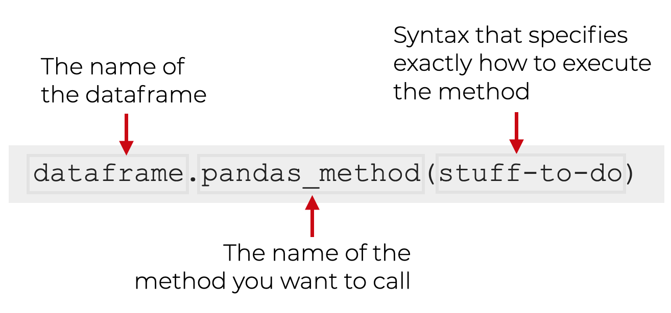
Then, inside the parenthesis for the method, you will have some code that’s unique to that method, and exactly how you’re using it.

With this general syntax in mind, let’s take a look at 5 specific Pandas methods that you should learn first.

The 5 most Important Pandas Methods

In my opinion, the most important data manipulation operations are:

• retrieving a subset of columns
• retrieving a subset of rows
• adding new variables
• sorting data
• aggregating data

That being the case, let’s look at the 5 Pandas methods that perform these:

• filter()
• query()
• assign()
• sort_values()
• agg()

There are quite a few other Pandas methods, but I strongly recommend that you learn these first. These are the tools that you’ll probably use the most often to wrangle your data.

Pandas Method Examples

Here, we’re going to take a look at examples of how to use filter(), query(), sort_values(), assign(), and agg().

Run this code first

Before you run any of these examples though, you’ll need to run some preliminary code first:

import pandas as pd
import seaborn as sns
import numpy as np

And also run the following:

titanic = sns.load_dataset('titanic')

Since we’ll be using Pandas, obviously you’ll need to import Pandas first.

But we’ll need some data to operate on, so here, we’ve used the sns.load_dataset() function to load the titanic dataset.

Ok, let’s start with the filter method.

FILTER()

One of the most common tasks in data science is subsetting columns.

For example, what happens if your dataset has too many columns, and you just want to work with a few of them?

Specifically, what if you want to retrieve a subset of columns by column name?

In Pandas, you can do this with the filter() method.

Let’s take a look.

Let’s say that you’re working with the titanic dataframe, which has 15 columns. With 15 columns, it’s sometimes a little difficult to print, and difficult to work with. And let’s say that for right now, you only want to look at 3 columns: sex, age, and survived.

You can do that as follows:

titanic.filter(['sex', 'age', 'survived'])

OUT:

        sex   age  survived
0      male  22.0         0
1    female  38.0         1
2    female  26.0         1
3    female  35.0         1
4      male  35.0         0
..      ...   ...       ...
886    male  27.0         0
887  female  19.0         1
888  female   NaN         0
889    male  26.0         1
890    male  32.0         0

[891 rows x 3 columns]

Explanation

Notice what happened here. The titanic dataframe has 15 columns. But when we use the Pandas filter method, it enables us to retrieve a subset of columns by name.

Here, we retrieved 3 columns – sex, age, and survived.

To retrieve these, we used so-called “dot syntax” to call the filter method with the code titanic.filter().

Then inside the parenthesis, we provided a list of the names of the columns that we wanted to retrieve: ['sex', 'age', 'survived'].

So when we use filter, we simply provide a list of column names and it will return that subset of columns. Notice that in the output, the columns are returned in the order they appear in the list … not in the order of the original dataframe.

Keep in mind that there are also other methods of subsetting columns, including the iloc method, which subsets rows and columns by numeric index. And also the loc method, which subsets rows and columns by label. These work differently from filter, however, so you should learn those tools separately.

In any case, there’s still more for you to learn about filter as well, so for more information on how to use filter(), check out our tutorial on the Pandas filter method.

QUERY()

Next, let’s take a look at the query() method.

The query retrieves rows of data.

More specifically, it retrieves rows that match some logical condition that you specify.

Let’s take a look at an example, and then I’ll explain.

Here, we’re going to retrieve rows for people who embarked from Southampton.

Let’s run the code:

titanic.query('embark_town == "Southampton"')

OUT:

     survived  pclass     sex   age  ...  deck  embark_town  alive  alone
0           0       3    male  22.0  ...   NaN  Southampton     no  False
2           1       3  female  26.0  ...   NaN  Southampton    yes   True
3           1       1  female  35.0  ...     C  Southampton    yes  False
4           0       3    male  35.0  ...   NaN  Southampton     no   True
6           0       1    male  54.0  ...     E  Southampton     no   True
..        ...     ...     ...   ...  ...   ...          ...    ...    ...
883         0       2    male  28.0  ...   NaN  Southampton     no   True
884         0       3    male  25.0  ...   NaN  Southampton     no   True
886         0       2    male  27.0  ...   NaN  Southampton     no   True
887         1       1  female  19.0  ...     B  Southampton    yes   True
888         0       3  female   NaN  ...   NaN  Southampton     no  False

[644 rows x 15 columns]

Explanation

Notice that the output has 644 rows of data instead of the original 891 rows from the full titanic dataframe. That’s because the output only contains rows where embark_town equals 'Southampton'.

How did we do this?

Here, we called the query() method using dot syntax.

Inside of the method, we used the logical expression 'embark_town == "Southampton"'.

Remember that embark_town is a column in the titanic dataframe. Additionally, Southampton is one of the values within that column.

So the expression 'embark_town == "Southampton"' instructs the query() method to retrieve only those rows where embark_town equals Southampton.

A couple extra notes on this …

First, the logical expression (i.e., 'embark_town == "Southampton"') must be enclosed inside of quotation marks. Single quotes or double quote will work. Essentially, the logical expression must be presented to query() as a string.

What that means is that if your logical expression contains a string value, you’ll need to use quotes for that string value as well. So if your logical expression is enclosed in single quotes, you need to enclose any string values in double quotes, or visa versa. (Effectively, you need to know how to work with strings to use query properly.)

Second, the logical condition that we used here was pretty simple. Having said that, it is possible to have fairly complex logical conditions.

Since there’s more to learn about this technique, you might want to check out our tutorial on the Pandas query method.

ASSIGN()

The assign method adds new variables to a dataframe.

To be clear, operations to create new variables can be simple, but they can also be very complex depending on what exactly you want your new variable to contain.

For the sake of simplicity and clarity, we’ll work with an extremely simple toy example here.

In this example, we’re going to create a variable called fare_10x.

Imagine that you’re working with the titanic dataset, and you find out that the fare variable is off by a factor of 10. You want to create a new variable that’s equal to the original fare variable, multiplied by 10.

You can do this with assign().

Let’s take a look:

titanic.assign(fare_10x = titanic.fare * 10)

OUT:

     survived  pclass     sex   age  ...  embark_town  alive  alone fare_10x
0           0       3    male  22.0  ...  Southampton     no  False   72.500
1           1       1  female  38.0  ...    Cherbourg    yes  False  712.833
2           1       3  female  26.0  ...  Southampton    yes   True   79.250
3           1       1  female  35.0  ...  Southampton    yes  False  531.000
4           0       3    male  35.0  ...  Southampton     no   True   80.500
..        ...     ...     ...   ...  ...          ...    ...    ...      ...
886         0       2    male  27.0  ...  Southampton     no   True  130.000
887         1       1  female  19.0  ...  Southampton    yes   True  300.000
888         0       3  female   NaN  ...  Southampton     no  False  234.500
889         1       1    male  26.0  ...    Cherbourg    yes   True  300.000
890         0       3    male  32.0  ...   Queenstown     no   True   77.500

[891 rows x 16 columns]

Explanation

Here, we’ve added a new variable to the output called fare_10x.

As I mentioned, this is equal to the value of the fare variable, times 10.

To create this, we simply called the .assign() method using “dot” syntax.

Then inside of the parenthesis, we provided the expression fare_10x = titanic.fare * 10. This is a “name/value” expression that provides the name of the new variable on the left-hand-side of the equal sign, and the value that we’ll assign to it on the right-hand-side.

Again, to be fair, this is a bit of a toy example. It’s possible to create much more complicated variables based on various logical conditions, and other operations.

For example, we can create a 0/1 indicator variable called adult_male_ind, which is 1 if the person is an adult male, and 0 otherwise (this is often called “dummy encoding”).

To do this though, we need to use a special function from Numpy called the Numpy where function.

titanic.assign(adult_male_ind = np.where(titanic.adult_male == True, 1, 0))

This is more complicated to do, and to accomplish it, you really need to know about Numpy.

All that being said, this example should get you started, but for more information, check out our tutorial on the Pandas assign method.

Additionally, if you want to become great at data manipulation, make sure to learn about Numpy!

sort_values()

Now, let’s look at the sort_values method.

The sort_values method sorts a dataframe.

This should be mostly self-explanatory, but let’s look at an example so you can see the method in action.

Here, we’re going to sort the titanic dataframe by the age variable.

titanic.sort_values(['age'])

OUT:

  survived  pclass     sex   age  ...  deck  embark_town  alive  alone
803         1       3    male  0.42  ...   NaN    Cherbourg    yes  False
755         1       2    male  0.67  ...   NaN  Southampton    yes  False
644         1       3  female  0.75  ...   NaN    Cherbourg    yes  False
469         1       3  female  0.75  ...   NaN    Cherbourg    yes  False
78          1       2    male  0.83  ...   NaN  Southampton    yes  False
..        ...     ...     ...   ...  ...   ...          ...    ...    ...
859         0       3    male   NaN  ...   NaN    Cherbourg     no   True
863         0       3  female   NaN  ...   NaN  Southampton     no  False
868         0       3    male   NaN  ...   NaN  Southampton     no   True
878         0       3    male   NaN  ...   NaN  Southampton     no   True
888         0       3  female   NaN  ...   NaN  Southampton     no  False

[891 rows x 15 columns]

By default, this sorted the data in ascending order.

We can also sort the data in descending order by setting ascending = False.

titanic.sort_values(['age'], ascending = False)

OUT:

     survived  pclass     sex   age  ...  deck  embark_town  alive  alone
630         1       1    male  80.0  ...     A  Southampton    yes   True
851         0       3    male  74.0  ...   NaN  Southampton     no   True
493         0       1    male  71.0  ...   NaN    Cherbourg     no   True
96          0       1    male  71.0  ...     A    Cherbourg     no   True
116         0       3    male  70.5  ...   NaN   Queenstown     no   True
..        ...     ...     ...   ...  ...   ...          ...    ...    ...
859         0       3    male   NaN  ...   NaN    Cherbourg     no   True
863         0       3  female   NaN  ...   NaN  Southampton     no  False
868         0       3    male   NaN  ...   NaN  Southampton     no   True
878         0       3    male   NaN  ...   NaN  Southampton     no   True
888         0       3  female   NaN  ...   NaN  Southampton     no  False

[891 rows x 15 columns]

Explanation

Here, we sorted the data by the age variable … first in ascending order, and then in descending order.

Just like all of these tools, we called sort_values using “dot” syntax. We typed the name of the dataframe, then .sort_values().

Importantly though, inside of the parenthesis, we provided a list of variables that we wanted to sort on. Here, we only sorted on age, so we passed in the Python list ['age'] as the argument.

Keep in mind, that you can pass in a list of multiple variables to sort the data on multiple variables.

For more examples of how to sort a Pandas dataframe, check out our sort_values tutorial.

AGG()

Finally, let’s look at the agg() method.

agg() summarizes your data.

For example, agg() can calculate the mean, median, sum and other summary statistics.

Let’s look at a simple example.

Here, we’ll calculate the means of our numeric variables.

titanic.agg('mean')

OUT:

survived       0.383838
pclass         2.308642
age           29.699118
sibsp          0.523008
parch          0.381594
fare          32.204208
adult_male     0.602694
alone          0.602694
dtype: float64

Explanation

Notice that the output contains the means of the numeric variables. It also includes the means of variables that can be coerced to numeric (although some, like the mean of adult_male, have unintuitive interpretations).

To call this method, we’ve simply used dot notation to call .agg(). Inside of the method, we’ve provided the name of a summary statistic, 'mean'.

Notice that the name of the statistic is being passed in as a string (i.e., it must be enclosed inside of quotations). Also take note that it’s possible to pass in a list of statistic names, like ['mean', 'median']. Uses of the agg method can get quite complex.

Remember: Pandas Methods almost always create a new dataframe

One quick note about these Pandas methods that we’ve looked at.

These Pandas methods create a new dataframe as an output.

What that means is that these data manipulation methods typically do not change the original dataframe. When we use these tools, the original dataframe remains intact.

This is really important, because that means that the changes that these methods make will not automatically be saved! This is really frustrating for beginners, who don’t understand what’s going on.

If you want to save the output, assign it to a variable

That being the case, you typically need to save the output of these Pandas methods, in one way or another.

If you want to save the output, you need to store the output in a variable name using the assignment operator.

Here is an example:

titanic_embark_southampton = titanic.query('embark_town == "Southampton"')

Alternatively, we could overwrite and update the original dataset, also using the assignment operator:

titanic = titanic.query('embark_town == "Southampton"')

But be careful when you do this.

If you re-use the name of your dataset like this, it will overwrite the original data. Although there are some cases where this is okay, there are other instances where you will want to keep your original dataset intact.

So again, be careful if and when you overwrite your data, and make sure that it’s exactly what you want to do.

How to “Chain” Pandas Methods Together

Now that you’ve learned about the 5 most important Pandas methods, let’s quickly talk about how to combine them together.

There’s a traditional way to do this, which I don’t like much at all.

There’s also a “secret” way to do it that is much easier to write, read, and debug (this secret way is actually similar to dplyr pipes in R).

Let’s talk about the traditional way first, and then I’ll show you the newer, better way.

The “Traditional” Syntax To Combine Pandas Methods

When you use Python methods, you can typically “chain” them together, one after another on a single line.

So let’s say that you want to first subset the rows where embark_town == "Southampton", but then you want to subset the columns to retrieve sex, age, and survived.

You can do this by typing the name of the dataframe, and then you can use “dot syntax” to first call the query method, and then call the filter method immediately after it, on the same line:

titanic.query('embark_town == "Southampton"').filter(['sex', 'age', 'survived'])

In this above code, we’ve called query() and filter(), in series, on the same line. The output will be a subsetted dataframe that subsets both the rows and columns.

This code works, but to me, there are some problems.

First, this code is extremely hard to read. It’s just too long moving horizontally. Everything sort of runs together.

Second, what if we wanted to use 3 methods in a row? What about 4? This doesn’t scale well.

And third, this code will be hard to debug. If you have a problem with any one of the methods that you use in series and you want to remove it from the chain, you need to delete that section, or make a copy of the code and delete the section you want to remove. Debugging code like this is a mess.

There’s got to be a better way, right?

Yes, and almost no one else will tell you how to do it.

But I’m a terribly generous guy, so I’ll show you the secret.

The “Secret” Chaining Syntax for Pandas

There’s actually a way to “chain” together multiple Pandas methods on separate lines.

The syntax is actually similar to how dplyr pipes work in the R programming language.

As an aside, I actually learned R before I learned Python. Although both are great languages, I actually think that R’s dplyr is better designed in many ways compared to Pandas.

One of the big reasons that I like R is that R’s Tidyverse functions are designed for using multiple functions in series, on separate lines. This is extremely useful for data wrangling and data analysis.

As soon as I started learning data science in Python, I wanted to replicate this behavior, but couldn’t find a way.

Eventually though, I discovered a simple way to do it, and my Pandas code has changed forever.

Pandas “Chain” Syntax

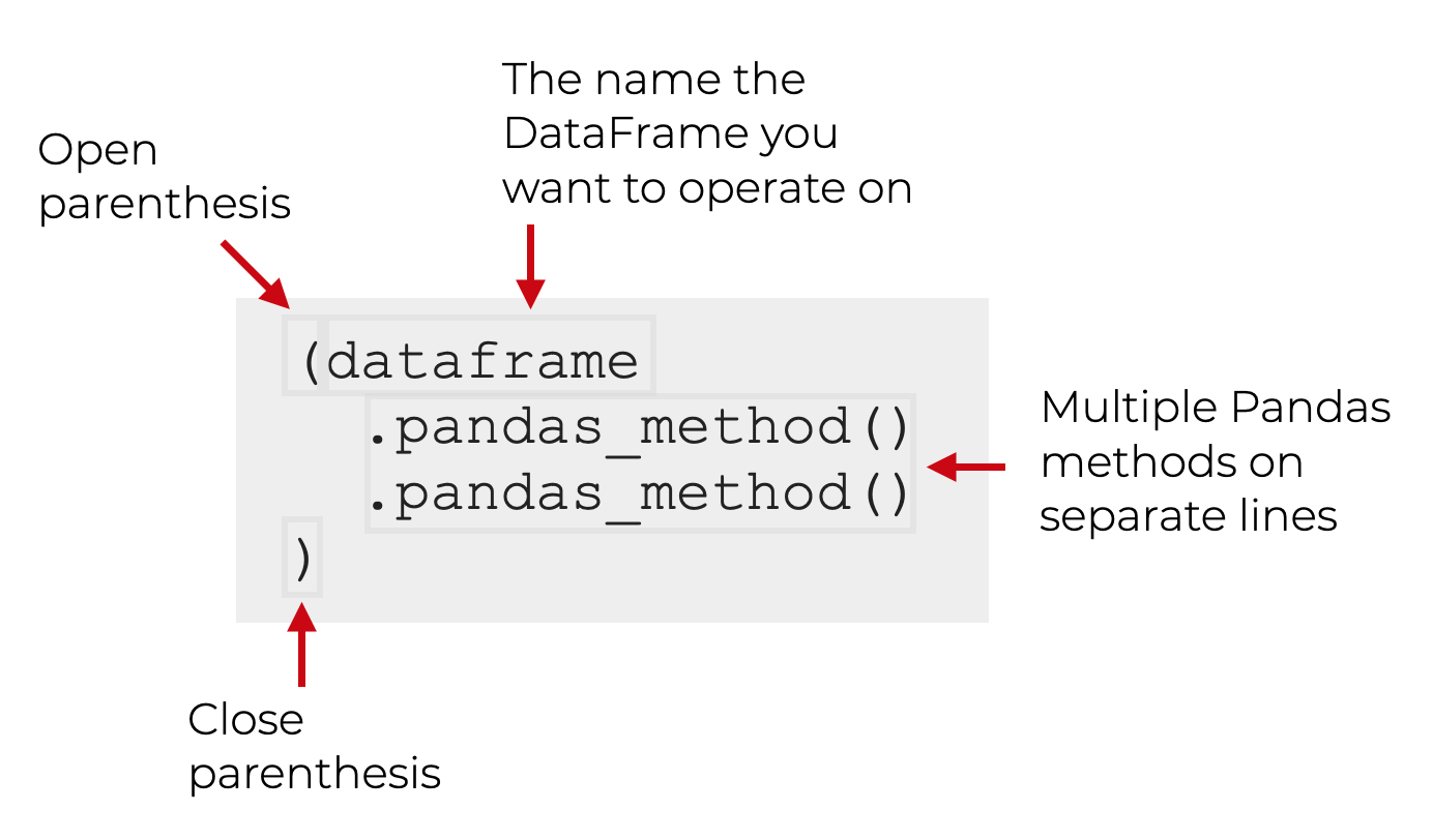
To create a “chain” of Pandas methods, you need to enclose the whole expression inside of parenthesis.

Once you do this, you can have multiple Pandas methods, all on separate lines. This makes writing, reading, and debugging your Pandas code much easier.

Here’s an example.

Let’s say that you want to use two Pandas methods, like we just did a couple sections ago. Let’s say that we want to first subset our rows with query, and then we want to subset the columns with filter.

Here’s how it will look with our special syntax:

This is a very powerful technique for manipulating your data. It enables you to do complex, multi-step data manipulations in an elegant way.

Before I show you an extreme case though, let’s look at a simple example.

A Simple Example of a Pandas Method Chain

Here, we’re going to re-do the “traditional” Pandas chain that we looked at a few sections ago.

First, we’re going to call query() and then we’ll call filter():

(titanic
 .query('embark_town == "Southampton"')
 .filter(['sex', 'age', 'survived'])
)

This is effectively the same as our previous code, which looked like this:

titanic.query('embark_town == "Southampton"').filter(['sex', 'age', 'survived'])

Both pieces of code will produce the same output.

The difference is that the this new version is much easier to read. Additionally, it’s easier to debug or modify.

For example, if you need to remove one of the methods, just put a hash mark in front of it to comment it out:

(titanic
 #.query('embark_town == "Southampton"')
 .filter(['sex', 'age', 'survived'])
)

Trust me, this is very convenient for debugging a chain of Pandas methods when you’re doing data manipulation.

It’s certainly useful even for simple chains of 2 methods, but it’s even more useful when you chain together multiple methods.

Multi-step Pandas chains

Using this chaining method, you can actually chain together as many Pandas methods as you want. You’re not limited to 2. You can do 3, 4 or more (although at some point, it will get a little ridiculous).

Let’s take a look at an example.

An Example of a Multi-step Dplyr Chain

Here, we’re going to do 3 operations:

• subset the rows where embark_town == "Southampton"
• subset the columns down to sex, age, and survived
• sort the data in descending order by age

Let’s take a look:

(titanic
 .query('embark_town == "Southampton"')
 .filter(['sex', 'age', 'survived'])
 .sort_values(['age'], ascending = False)
)

OUT:

        sex   age  survived
630    male  80.0         1
851    male  74.0         0
672    male  70.0         0
745    male  70.0         0
33     male  66.0         0
..      ...   ...       ...
846    male   NaN         0
863  female   NaN         0
868    male   NaN         0
878    male   NaN         0
888  female   NaN         0

[644 rows x 3 columns]

Here, we did a somewhat complex, multi-step data manipulation with code that’s relatively easy to read and easy to work with.

And as I mentioned, we could actually add more methods if we needed to!

Read Each Line as as ‘then’

One additional comment about this multi-line chaining syntax.

When you read this code, you read each line with a “then”.

Let’s look at out multi-line chaining code again, and I’ll add some comments to show you what I mean.

(titanic                                    # Start with the titanic dataset
 .query('embark_town == "Southampton"')     # THEN retrieve the rows where embark_town equals Southampton
 .filter(['sex', 'age', 'survived'])        # THEN retrieve the columns for sex, age, and survived
 .sort_values(['age'], ascending = False)   # THEN sort the data by age in descending order
)

We can read this code line-by-line as a series of procedures.

In my opinion, writing your code this way makes it 10X easier to read.

You should start doing this. It will make your code easier to write, easier to debug, and easier to read.

Perform complex data manipulation with Pandas chains

In addition to readability, using these multi-line Pandas chains makes it much easier to do complex data manipulations.

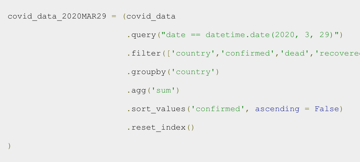
For example, in a previous tutorial series, we wrangled and analyzed covid-19 data. In one part of that analysis, we chained together 6 different Pandas tools.

Doing data manipulation this way is extremely powerful. Once you master this technique, you’ll never go back.

It’s simple, powerful, and quite honestly, a joy to use.

You Need to Master the Python Pandas Package

Hopefully, this introduction to the Python Pandas package was helpful.

Data manipulation is a critical, core skill in data science, and the Python Pandas package is really necessary for data manipulation in Python. Like it or not, you need to know it if you want to do data science in Python.

Having said that, there’s a lot that this tutorial didn’t cover. There’s a lot more to learn about Pandas.

If you want to dive deeper into other parts of the Pandas package, and on data manipulation generally, check out these other tutorials:

• An Introduction to Pandas dataframes
• 3 Secrets for Mastering Data Manipulation
• Why data manipulation is the foundation of data science
• The 19 Pandas functions you need to memorize

Essentially, even though this tutorial should get you started, there’s a lot more to learn. Once you master all of the essentials of Pandas, you’ll be able to do much, much more.

Leave your Questions in the Comments Below

Do you have questions about the Python Pandas package?

Is there something that you don’t understand, or something you think I missed?

If so, leave your question in the comments section near the bottom of the page.

Enroll in our course to master Pandas

If you’re really ready to master Pandas, and master data manipulation in Python, then you should enroll in our premium course, Pandas Mastery.

Pandas Mastery will teach you all of the essentials you need to do data manipulation in Python.

It covers all of the material in this tutorial, and a lot more. It will teach you all of most important Pandas methods (a few dozen), and how to combine them.

But it will also show you a unique training system that will help you memorize all of the syntax you learn, and become “fluent” in Python data manipulation.

If you’re serious about mastering data manipulation in Python, and you want to learn Pandas as fast as possible, you should enroll.

We’re reopening Pandas Mastery next week, so to be notified as soon as the doors open click here and sign up for the waiting list:

Yes! Tell Me When Pandas Mastery Opens Enrollment