A Quick Introduction to the Seaborn Objects System

Have you ever been frustrated with data visualization in Python?

Matplotlib – as powerful as it is – has a very clumsy syntax. It’s hard to use.

Plotly is OK, but still feels complicated for more advanced visualizations.

Personally, I’ve been frustrated with the data visualization options in Python, and I’ve been waiting for a powerful visualization toolkit that has a simple, easy-to-understand syntax.

The wait is over.

My New Favorite Toolkit for Python Data Visualization

The new Seaborn Objects system has just been released, and I think it is the best, most powerful, most user friendly data visualization system for Python.

Interested? Keep reading.

This tutorial will introduce you to the new Seaborn Objects system for Python data visualization.

It will cover most of the basics of how to use the new Seaborn Objects system, and will show you some examples of how to use it.

If you need something specific, you can click on any of these links to go to the appropriate section in the tutorial.

Table of Contents:

• What is the “Seaborn Objects” System?
• The Syntax of the Seaborn Objects System
• Examples of How to Use the Seaborn Objects System

Now keep in mind that the Seaborn Objects system is very new, and it represents a fundamental change in how we create data visualizations in Python using Seaborn.

That being the case, I strongly recommend that you read the full tutorial. You’ll get a much better understanding if you do.

What is the “Seaborn Objects” System?

Let’s start with the basics.

Here, we’ll talk about Seaborn at a high level, where it fits into the Python data science ecosystem, and also what this new “objects” system is all about.

Seaborn is a Data Visualization Package for Python

You might be familiar with Seaborn, and you probably know that Seaborn is a data visualization package for Python.

Seaborn was introduced several years ago, as an alternative to Matplotlib (although, to be clear, it’s actually built on top of Matplotlib).

In the initial form, Seaborn provided a variety of functions for creating most essential data visualizations: scatterplots, line charts, bar charts, histograms, heatmaps, etc.

And to be honest, most of these basic visualizations look pretty good.

And the syntax for those visualizations is pretty easy to use.

But, the original Seaborn package has limits.

The Original Seaborn Package Has Limits

Even though the Original Seaborn package was pretty good, it was still somewhat limited.

First, more advanced visualizations were challenging to create.

If you needed to create a multi-layer plot with multiple datasets, you’d probably have a difficult time.

Additionally, a lot of the formatting for Seaborn plots needed to be performed with Matplotlib, which is difficult to use.

Ultimately Seaborn was great at creating most basic to low-intermediate plots, but for anything really complicated, Seaborn seemed to hit a limit.

The Original Seaborn Lacked Flexibility

Ultimately, the old Seaborn system lacked flexibility.

It was easy to create a straightforward scatterplot or bar chart, but if you needed to create something more complicated, the original Seaborn often lacked the necessary flexibility.

This is in contrast to some other data visualizations packages like R’s ggplot2, or Tableau, which are both extremely flexible and easy to use.

To be honest, I have been waiting for a data visualization system in Python that had similar power, flexibility, and simplicity to ggplot2.

Well, now it’s here.

The Seaborn Objects System is a New Data Visualization System for Python

The Seaborn Objects system is a new way to create data visualizations in Python.

This new system was released recently in early September 2022, as part of the v0.12 Seaborn release.

It provides an all new way to create data visualizations in Python.

The Seaborn Objects System is a Simple, Flexible, and Powerful Data Visualization Toolkit

The new Seaborn Objects system provides an all new syntax for creating data visualizations in Python.

And it’s simple, powerful, and flexible.

There are a few specific things that make it so useful and user friendly.

The Seaborn Objects System works Well With Dataframes

First, the Seaborn Objects system works natively with dataframes.

This is in contrast to some of the other Python data visualization packages.

For example, Matplotlib sometimes works poorly with dataframes. Some Matplotlib functions work OK with dataframes (i.e., the Pyplot functions).

But in other cases, Matplotlib requires you to use things like for-loops to plot data in a dataframe. This makes using Matplotlib challenging, especially for beginners.

Plotly also feels a little clumsy when working with dataframes.

Again, the new Seaborn system works great with dataframes (and it also works with other structures like Numpy arrays).

The Seaborn Objects System is Highly Modular

The Seaborn Objects system takes a different approach to data visualization than tools like Matplotlib, Plotly, and even the “original” Seaborn.

The Seaborn Objects system is modular. You create a plot by calling functions and methods and putting them together like building blocks.

So instead of calling a “scatterplot” function to create a scatterplot, you call a generalized “plot” function, and then tell it to add “dots” to the plot.

Or instead of calling a “barplot” function, you call a generalized “plot” function, and then use a different function to add bars.

To get a little technical here, this new visualization system is based on the Grammar of Graphics, a theoretical framework that has influenced other powerful visualization toolkits like ggplot2 and Tableau.

The Seaborn Objects System has a Highly Structured Syntax

Finally, the syntax is highly structured.

As noted above, the system is highly modular. You create new charts by calling additional functions and methods to make little modifications to your plot.

So there’s one generalized “plot” function.

There’s a generalized method that allows you to “facet” a plot into different windows.

There are generalized methods that allows you to modify the labels and scales.

So ultimately, the syntax to create a visualization is often very similar whether you’re creating a bar chart, line chart, or any other visualization.

There’s a structure and uniformity to how you create different visualizations which simplifies the process of doing data visualization in Python.

With all that said, let’s start looking at the syntax. Once you see the syntax, it will start to become clear what I mean when I say that the system is “modular”. And in turn, you’ll begin to see why it’s so simple, yet powerful.

The Syntax of the Seaborn Objects System

Here, we’ll talk about the syntax of the Seaborn objects system.

Before we get into it, let me be clear: this is entirely new syntax in Seaborn. Even if you’re familiar with traditional syntax, the vast majority of this will be new to you.

The High-Level Syntax

The Seaborn Objects syntax is different from traditional Seaborn syntax, in that it works in a modular way.

Instead of having one function for scatterplots, one for bar charts, one for line charts, etc, the new system has little “building” blocks that you can put together in different ways to create different visualizations.

At a high level though, syntactically, there are a few parts that you’ll see in almost every visualization:

• the Plot function
• the add method
• a function that adds marks to a plot

To be clear there are other pieces of the Seaborn Objects syntax, like the facet() method, scale() method, theme() method, and others. But here, I want to stick to the most important components of the Seaborn Objects syntax.

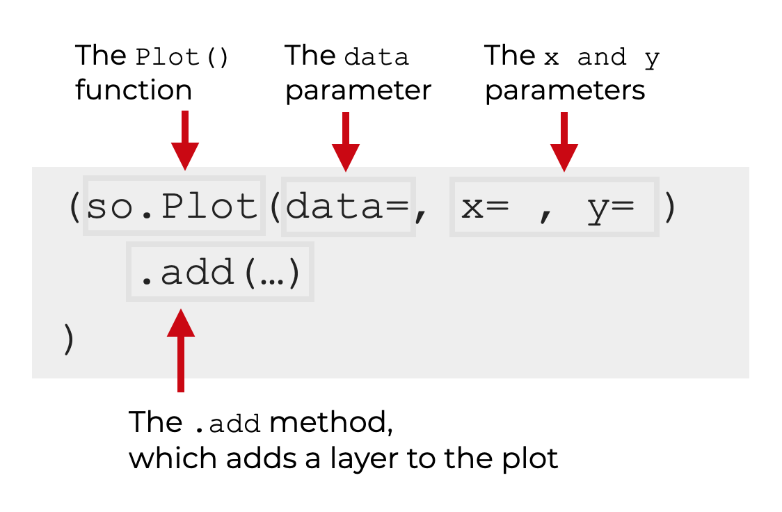
The Seaborn “Plot” function

The so.Plot() function is fairly simple.

This function initiates plotting for a Seaborn Objects plot.

Technically, you can call this function all by itself.

For example, run this code:

so.Plot() 

And it will create an empty plot:

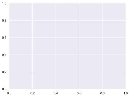
You’ll need to use this function for any Seaborn Objects visualization.

The Plot Function has Parameters for the Data and “Mappings”

Inside of the plot function, there are some parameters.

Some of these parameters will be optional, but a few are commonly used.

Most importantly, you’ll find:

• the data parameter
• the x parameter
• the y parameter
• the color parameter

There are also some parameters that are important for some plots, but less commonly used, like the group parameter.

Let’s quickly review what the above parameters do.

data

The data parameter specifies the dataframe that you want to use from the plot. The argument to this parameter will be a Pandas dataframe.

This parameter is optional, but it will be common with most Seaborn Objects plots.

Essentially, if the data that you want to plot exists as columns in a Pandas dataframe, you need to use this parameter.

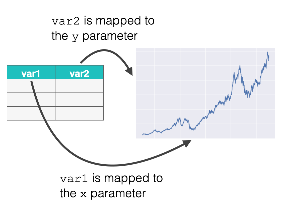
x and y

The x and y parameters specify the data that you want to “map” to the x and y axes of your plot.

Most plots will use at least one or the other of these parameters.

Some plots, like histograms, may only use one. A histogram will typically only use the x parameter.

Other plots, like scatterplots, will use both of them.

Whether you use the x or y parameters, and how exactly you use them, will depend on the exact plot you’re trying to make.

The arguments to these parameters depends on the data structure that stores your data.

Most commonly, if you’re plotting columns in a Pandas dataframe, the arguments to these parameters will be the names of the columns. When the argument is the name of a dataframe column, the column name must be enclosed inside of quotes.

Alternatively, you can also plot data in a Numpy array. In this case, you’ll pass the name of the array to the x or y parameter (without quotes).

color

The color parameter allows you to map a variable to the color of the marks.

For example, if you have different categories in your data, you can map a categorical variable to the color parameter to plot the different categories as different colors:

(so.Plot(data = stocks
         ,x = 'date'
         ,y = 'close'
         ,color = 'stock'
         )
   .add(so.Line())
 )

OUT:

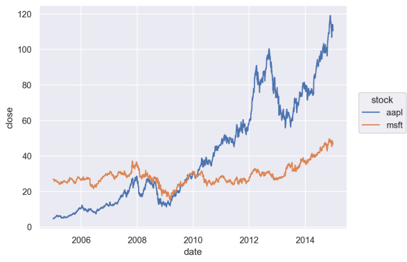
The color parameter can be used with categorical data as well as numeric data.

Adding “Marks”

When you create a Seaborn Objects plot, you need to select the type of mark that you want to draw.

For example, you can draw “dots”, “lines”, or “bars.”

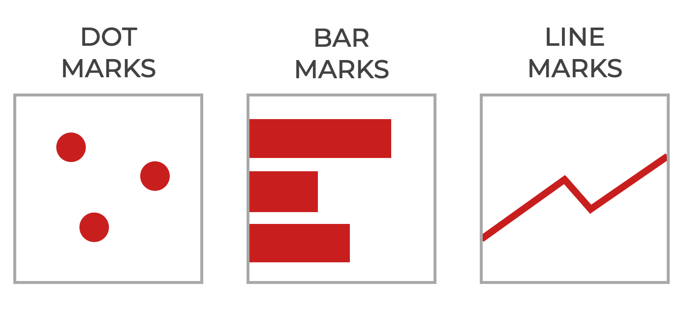
Dots, lines, and bars are all types of “marks” in the Seaborn Objects system.

But there are also other types of marks, such as “area” marks (which create area plots) and “range” marks. Most of these marks are less commonly used.

To add a mark, you call a mark function inside of the .add() method, as seen here:

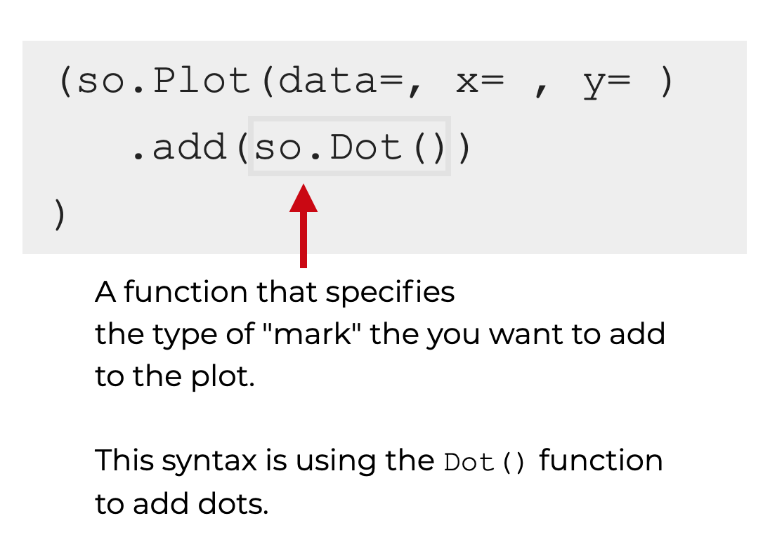
So to add “dots” you’ll call so.Dot().

To add lines, you’ll call so.Line().

Moreover, the type of mark that you add, along with how you map your data to the plot, determines the type of plot that you create. For example, to make a scatterplot, you need to add “dot” marks.

Adding Multiple Layers

You can also add multiple layers of marks to your plot.

This is where the Seaborn Objects system really shows its power and flexibility.

To add multiple layers, you simply call the add method multiple times. Inside each separate call, you specify what mark you want to plot.

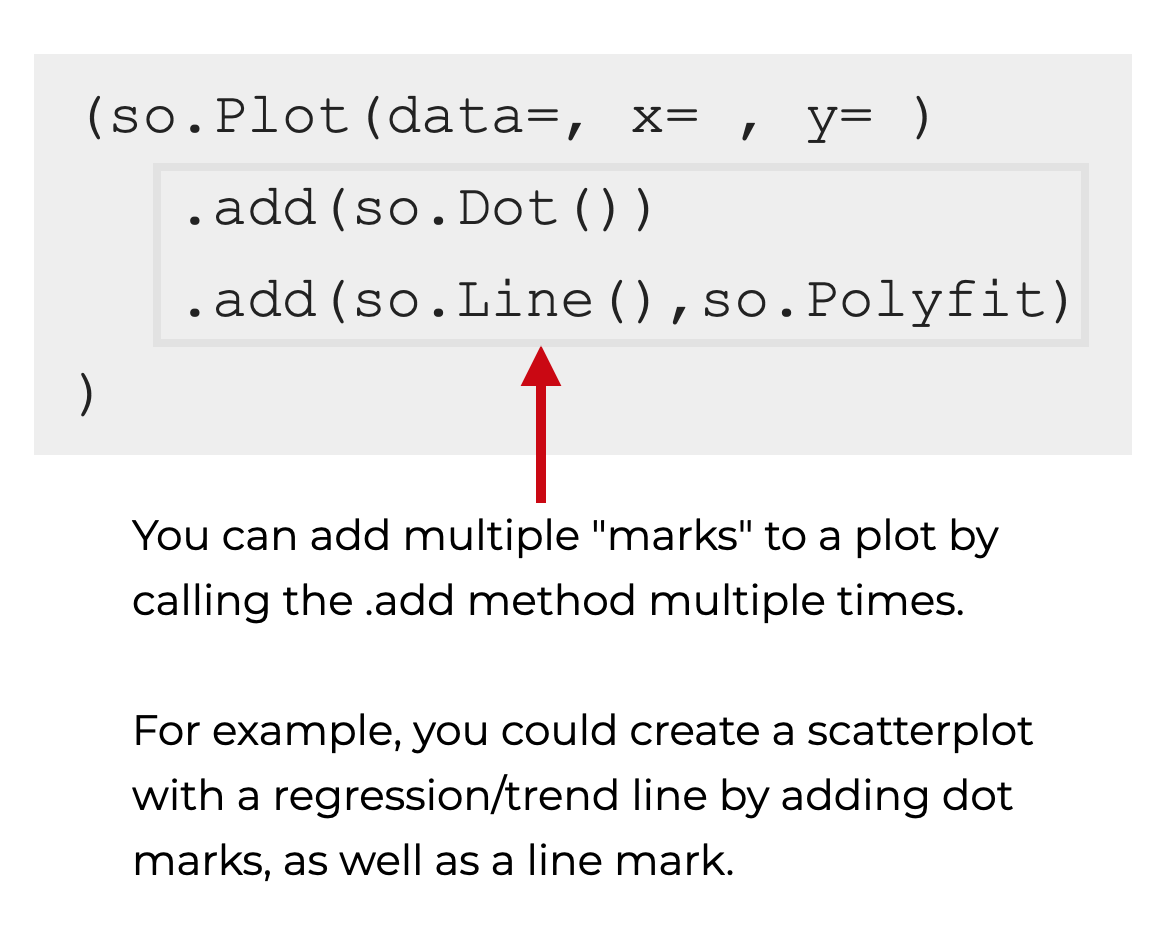
Importantly, each of these new layers will use the variable mappings that you specify in the call to so.Plot() by default.

Examples of How to Use The Seaborn Objects System

Now that we’ve looked at the syntax, let’s look at some examples of how to use the Seaborn objects system to create some basic charts and graphs.

Examples:

• How to create a scatterplot
• How to create a line chart
• How to create a bar chart

Run this code first

Before you run the examples, you’ll need to run some setup code first.

Import Packages

First, you need to import some packages.

We’ll need to import base seaborn (mostly to get some data), and we also need to import the Seaborn Objects subpackage.

Additionally, we’ll import Pandas, because we’ll need it to retrieve a dataframe.

import seaborn as sns
import seaborn.objects as so
import pandas as pd

Once you import these, you’ll be read to go.

EXAMPLE 1: Create a scatterplot

First, we’ll create a scatterplot.

Let’s run the code first, and then I’ll explain.

Get Data

First, we need to get the data that we’ll use.

Here, we’ll plot variables in the supercars dataframe, which we’ll get with the Pandas read_csv function.

supercars = pd.read_csv('https://learn.sharpsightlabs.com/datasets/pdm/supercars.csv')

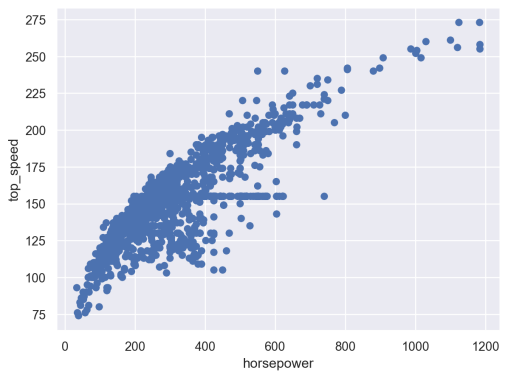
Create Scatterplot

Here’s the Seaborn Objects code to create a scatterplot from our supercars data:

(so.Plot(data = supercars
         ,x = 'horsepower'
         ,y = 'top_speed'
         )
   .add(so.Dot())
 )

OUT:

Explanation

So let’s break this down.

To initialize the plot, we called so.Plot().

Inside of the call to so.Plot(), we used the data parameter to specify that we want to plot data from the supercars dataframe.

We specified that we want to put the horsepower column on the x-axis, and the top_speed column on the y-axis. Notice that the names of these columns are enclosed inside of quotation marks. That’s because they are names of columns inside of our dataframe.

We’re using the .add() method to add our mark type. Because this is a scatterplot, we’re using so.Dot() to add dot marks.

That’s it!

Specify the data source. Specify the variable mappings. Specify the mark type.

Notice as well that the whole expression is enclosed inside of parenthesis. That allows us to put all of the different method calls on separate lines. It’s just a way to make our code easier to read.

EXAMPLE 2: Create a Line Chart

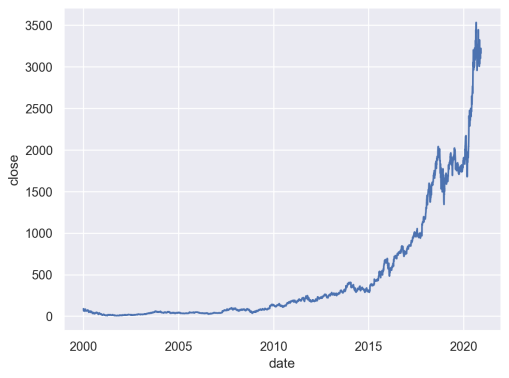
In this example, we’re going to plot Amazon stock price data.

Get Data

First, we need to get the data that we’re going to plot by downloading some stock data with Pandas read_csv.

Then we’ll do some processing with the Pandas to_datetime method, and we’ll use the Pandas query method to create a subset of only Amazon stock.

stocks = pd.read_csv("https://www.sharpsightlabs.com/datasets/amzn_goog_2000-01-01_to_2020-12-05.csv")
stocks.date = pd.to_datetime(stocks.date)
amazon_stock = stocks.query("stock == 'amzn'")

Create Scatterplot

Now, we’ll use Seaborn Objects to create the line chart.

(so.Plot(data = amazon_stock
         ,x = 'date'
         ,y = 'close'
         )
   .add(so.Line())
 )

OUT:

Explanation

If you understood example 1, this should make sense, because it’s structurally almost identical.

We called the so.Plot() function to initialize the plot.

We specified the dataframe that we want to plot with the data parameter, and mapped the appropriate variables to the x and y axes.

Then we called the .add() method with so.Line() to specify that we want to draw lines.

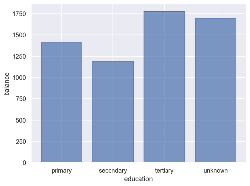
EXAMPLE 3: Create a Bar Chart

Finally, let’s create a bar chart.

Get Data

In this example, we’ll use some bank data, that we’ll once again retrieve with Pandas read_csv.

bank = pd.read_csv('https://learn.sharpsightlabs.com/datasets/pdm/bank.csv')

Create Bar Chart

Here, we’ll create a bar chart of bank balance, by different level of education:

(so.Plot(data = bank
         ,x = 'education'
         ,y = 'balance'
         )
   .add(so.Bar(), so.Agg())
 )

And here’s the resulting chart:

Explanation

Structurally, you’ll notice that the syntax for this chart very similar to the syntax for the scatterplot and line chart.

We call the so.Plot() function to initialize the visualization.

We specify the dataframe that contains the data we want to plot, and map the appropriate variables to the x and y axes.

Then we use the .add() method to add bar marks with so.Bar(). Note as well that we need to use so.Agg() to aggregate the data. By default, this function computes the mean. So here, it’s computing the mean balance by education.

There’s Still More To Learn About Seaborn Objects

In this tutorial, I’ve shown you some of the high-level basics of the Seaborn objects system.

But there’s more to learn.

I’m going to publish separate tutorials about:

• How to modify labels and titles
• How to create small multiple chart (i.e., faceting)
• How to create pair plots
• How to create multi-panel plots
• How to modify the “theme” properties of Seaborn Objects plots
• and more

For more data science tutorials, sign up for our email list

If you want to learn more about Seaborn and other data science tools, sign up for our email list.

Here at Sharp Sight, we teach data science.

Every week, we publish articles and free tutorials about data science.

If you sign up for our email list, you’ll get these tutorials delivered right to your inbox.

You’ll learn about:

• Seaborn
• Pandas
• Numpy
• Scikit Learn
• data science in R
• … and more.

Want to learn data science? Sign up now.