Dealing with the problem of overfitting is one of the core issues in machine learning and AI.
Your model seems to work perfectly on the training set, but when you try to validate it on the test set … it’s terrible.
This is a core problem in machine learning, especially when you start using advanced ML techniques like deep learning.
And to solve the problem of overfitting, you often need regularization.
Regularization is one of the primary tools that we use to build models that fit the data well, but also generalize well to unseen data.
So in this blog post, I’m going to explain the essentials of regularization.
I’ll explain what regularization is and also introduce you to the primary types of regularization.
If you need something specific, you can click on any of the links below, and the link will take you to the appropriate location in the article.
Table of Contents:
A Simple Explanation of Regularization
Put simply, regularization is a modification to a machine learning algorithm that increases its ability to generalize.
Said differently, regularization techniques modify how a machine learning algorithm learns in a way that decreases overfitting.
A Quick Review of Overfitting
Overfitting occurs when a model fits too closely to the training data. This typically happens when the model is too flexible, and that flexibility enables it to “flex” to reduce all of the training error.
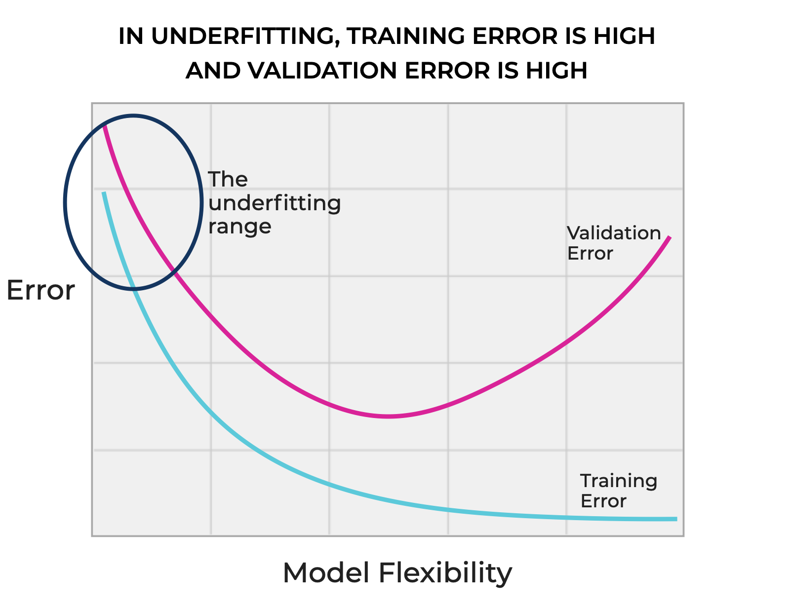
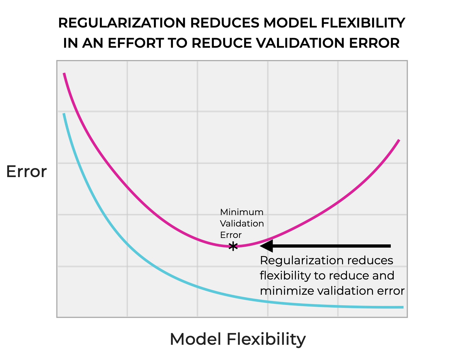
You can think of this in terms of how model error relates to model flexibility.
In the underfitting range, model flexibility is low, which in turn causes both training error and validation error to be high.
On the other hand, in the overfitting range, model flexibility is high, which enables the model to “flex” to reduce the error on the training set. This means that the training error is very low, but because the model is fit to closely too the noise or specific patterns in the training data, the validation error will be high.
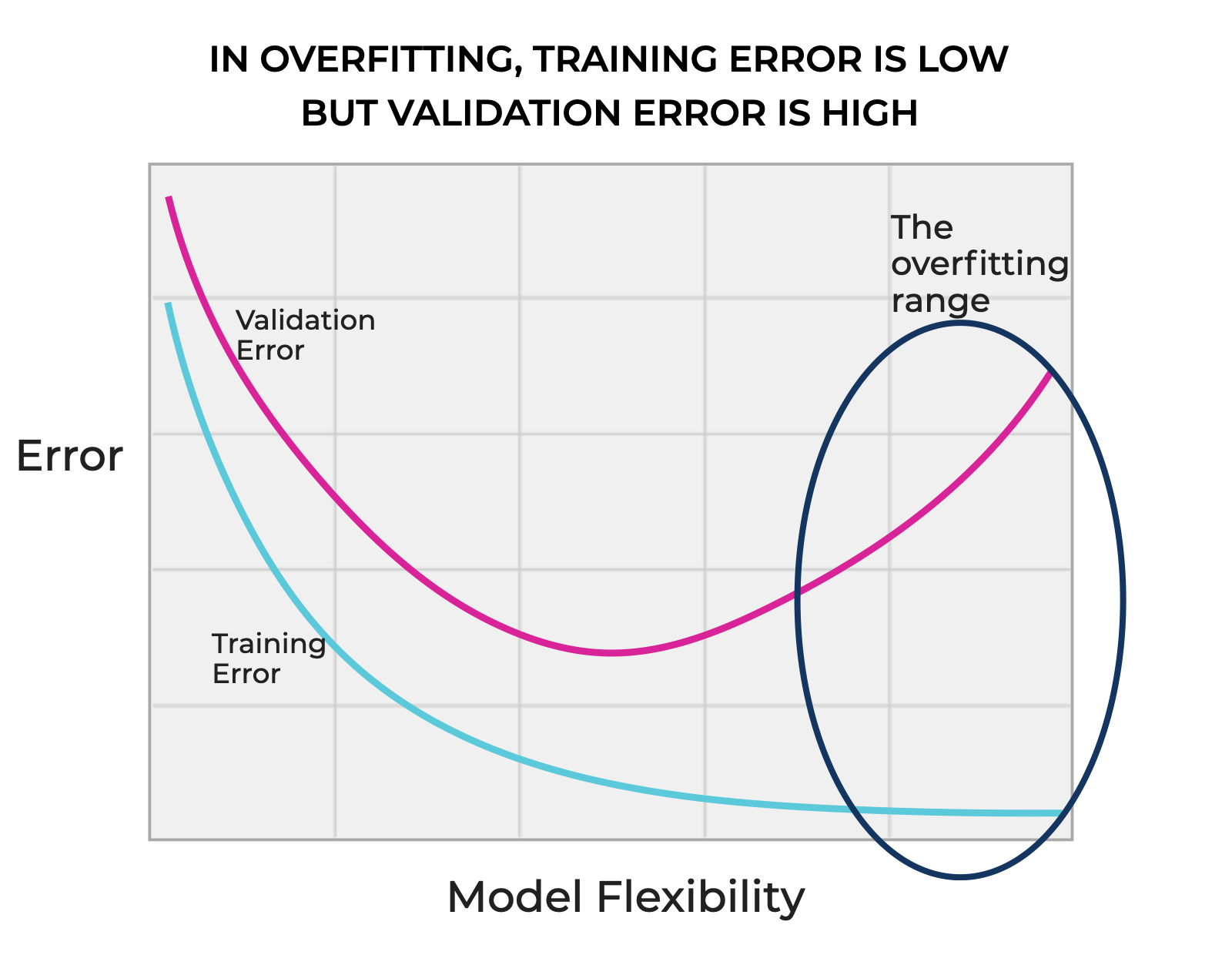
In the most extreme case, a model that’s overfitting will exactly hit all of the training points, resulting in very low training error, but a substantial validation error.
A Visual Example of Overfitting and Underfitting
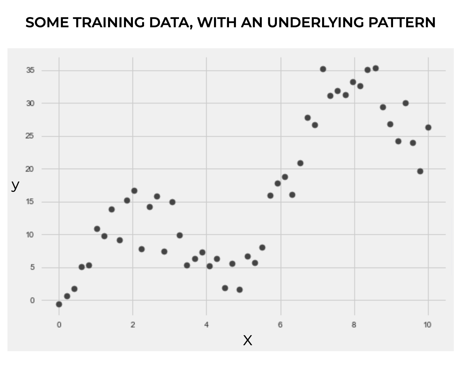
Let’s look at a quick example.
Here, we have a simple dataset with one feature (the  variable) and the target (the
  ) variable.
If you look at the data, there’s a pattern. The actual pattern is a linearly increasing sine wave, with some added noise.
When we’re doing machine learning, we build a computer system based on a learning algorithm, and we try to get the system to learn what the pattern in the data by exposing the system to data examples.
It’s getting a computer system to learn what the underlying function is that generated the data, by exposing the system to datapoints generated by that function.
But machine learning algorithms are imperfect.
They can overfit, which is seen in the highly flexible model below that hits all of the training points.
Or they can underfit, which we see in the straight line which poorly fits the data.
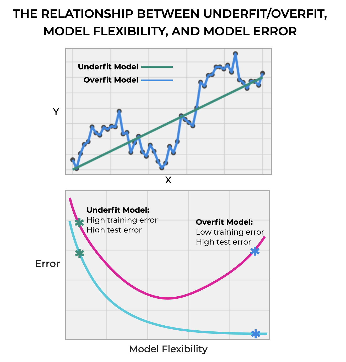
Underfitting is bad, because it means that the model inadequately models the training data. The result of this (as seen in the second chart just above) is that both training error and test error are high. It’s a bad fit for both the training data and test data.
But overfitting is bad because it follows the “noise” in the training data too much, which in turn, makes it hard for the model to generalize to new, previously unseen data. The result of overfitting, is that the training error is very low, but the test error is high (i.e., the model overfits the training data, but is a bad fit for previously unseen data).
Striking a balance between underfit and overfit is one of the core problems in machine learning. It is at the heart of training AI and machine learning systems.
Managing Overfitting is Core Problem of Machine Learning
Importantly, as problems get more complicated, we often need to use more powerful techniques that are flexible enough to find more complex patterns in the data.
For example, in many complex, real-world problems, we need very flexible techniques such as gradient boosted trees or deep neural networks.
These powerful techniques are flexible enough to find complex patterns in the training data, but, as flexibility increases, the risk of overfitting increases.
How do we solve this?
One of the main ways is with regularization.
Regularization Mitigates Overfitting
Regularization techniques provide a way to control the complexity (i.e., flexibility) of a model.
Regularization attempts to reduce the flexibility of the model in order to reduce the validation error. Ideally, we’re trying to build a model that minimizes the validation error (as opposed to minimizing the training error).
In terms of the bias/variance tradeoff, adding regularization reduces model variance, thereby decreasing the likelihood of overfitting (but which increases bias).
So regularization decreases the flexibility (i.e., variance) of the model, which reduces the problem of overfitting, ensuring that the model generalizes well to previously unseen data.
In turn, this enables better performance and better predictions on new data.
Main Types of Regularization
Now that we’ve discussed what regularization is at a high level, let’s get into some of the details of particular, commonly used forms of regularization.
The main techniques that I want to cover are:
- L1 regularization (LASSO)
- L2 regularization (Ridge)
- Elastic Net
I’ll also mention a few more, briefly towards the end of this section, like dropout and early stoppage.
L1 regularization (LASSO)
First, let’s talk about L1 regularization.
L1 regularization, which is also called LASSO (meaning Least Absolute Shrinkage and Selection Operator) adds a penalty to the loss function equal to the absolute value of the weights of the model.
Mathematically, if the original loss function of the model is  , and the model has parameters
  , then we can define the L1 regularized loss function as:
(1) 
Where  is the strength of regularization (i.e., the regularization parameter).
Use Cases and Advantages
L1 regularization is particularly useful for feature selection, because it tends to push some of the model coefficients to exactly zero. This has the effect of removing some features completely from the model.
This is especially useful when you have high-dimensional data (i.e., a lot of features in your data), but when some of those features are redundant or irrelevant.
The ability to reduce model complexity by eliminating some features makes it useful not only to reduce overfitting, but also increase computational efficiency and model interpretability.
L2 Regularization (Ridge)
L2 regularization – also called Ridge or Ridge regression – adds a penalty to the loss function equal to square of the magnitude of the weights of the model.
Mathematically, L2 is somewhat similar to L1.
We take the original loss function of the model, , and if the model has parameters , then we can define the L2 regularized loss function as:
(2) 
Again, where , the regularization parameter, is the strength of regularization.
Use Cases and Advantages
The effect of L2 regularization is somewhat different than L1.
Whereas in L1, where the regularization tends to shrink some of the coefficients to zero, L2 regularization (Ridge) tends to keep all of the features shrink all of the coefficients somewhat (typically, none of the coefficients are reduced to exactly zero). So Ridge tends to keep all of the features, but it “shrinks” their effect on the model.
Ridge regression is particularly useful when the features have high multicollinearity (i.e., when features are highly correlated).
By shrinking the coefficients, L2 reduces the variance of the model and improves model stability.
Ultimately, L2 regularization is most useful in situations where we need to reduce overfitting, but we also want to keep all of the features in the model (although, with reduced influence).
Elastic Net Regularization
Elastic net is a hybrid regularization technique that combines both L1 and L2 regularization.
Specifically, in Elastic Net, we add both regularization penalties from L1 and L2.
So if we have the original loss function , and model parameters , then we can define the Elastic Net regularized loss function as:
(3) 
Where  is the strength of the L1 regularization and
  is the strength of the L2 regularization.
Use Cases and Advantages
Elastic Net is particularly useful when the model has a large number of features that are correlated with each other.
It combines the feature elimination properties of L1 regularization with the broad reduction in feature importance from L2.
Elastic Net works best when you have a complex dataset where you need to eliminate some features, while also broadly reducing remaining effects of collinearity between the remaining features to reduce overfitting.
Essentially, Elastic Net balances between L1 and L2. Whereas L1 alone regularization can be overly aggressive in removing features and L2 regularization can be insufficient if there are totally irrelevant features that should be removed, Elastic Net enables you to tune the regularization to provide varying amounts of L1 and L2, depending on the problem you’re working on.
The main tradeoff then is that while Elastic Net can provide more nuanced regularization that combines L1 and L2 effects, Elastic Net is harder to tune, and may be more computationally expensive.
Other Types of Regularization
Beyond L1, L2 and Elastic Net, there are other types of regularization.
A few that you might want to know about – particularly for neural networks – are dropout and early stoppage.
Dropout
Dropout is primarily used in deep neural networks.
In dropout regularization, during every step of the training process, neurons are randomly selected and ignored (i.e., dropped out) with a certain probability.
By randomly dropping some of the neurons during every different training step, dropout regularization limits the network’s reliance on a small number of neurons. In turn, forces the model to learn more robust representations.
This regularization technique is particularly useful for large and complex deep networks.
Early Stoppage
In early stoppage, the regularizer stops training before model fully converges.
It does this by monitoring the performance of the model on the validation set, and it stops training the model once the validation performance stops improving.
By stopping training when the validation performance ceases to improve, this regularization technique stops the model from overfitting to the noise in the data (which is the core problem in overfitting).
A Final Note on Different Regularization Techniques
Every regularization technique has specific advantages and disadvantages, and in turn each technique has specific use cases.
The choice of regularization technique depends on the task you’re trying to perform, the nature of the dataset, the features, the cause(s) of overfitting, etcetera.
All that said, regularization is critical for preventing overfitting. And because overfitting is one of the core problems in building robust learning systems, you need to know how to use different regularization techniques, and when to use one technique over another.
Wrapping Up
Regularization is a really big topic.
In this post, I tried to give you a high-level overview of regularization, but I want to write a lot more about this subject in the future.
In particular, I’ll write more about:
- How to implement regularization in Python with Scikit Learn
- How to choose the best regularization technique for a particular problem
- An in depth review of L1 regularization
- An in depth review of L2 regularization
- How regularization relates to the bias/variance problem
- A review of regularization technique for deep learning
And more.
Sign Up for our Email List
If you want to learn more about regularization specifically, and if you want to learn more about machine learning and AI specifically, then sign up for our email list.
When you sign up, you’ll get free tutorials on:
- Scikit learn
- Machine learning
- Deep learning
- Generative AI
- Machine learning engineering
- Data analytics
And more.
We publish tutorials for FREE every week, and when you sign up for our email list, they’ll be delivered directly to your inbox.
Great post! Thanks!
I’m looking forward to the detailed implementations in the next post.
János
Many thanks.