How to Use geom_smooth in R

This tutorial will show you how to use the geom_smooth function in R.

It explains what geom_smooth does, explains the syntax, and shows step-by-step examples of how to use this function.

If you need something specific, you can click on any of the following links. These links will take you directly to the appropriate place in the tutorial.

Table of Contents:

• Introduction
• Syntax
• Examples
• Frequently Asked Questions

A quick introduction to Geom Smooth

The geom smooth function is a function for the ggplot2 visualization package in R.

Essentially, geom_smooth() adds a trend line over an existing plot.

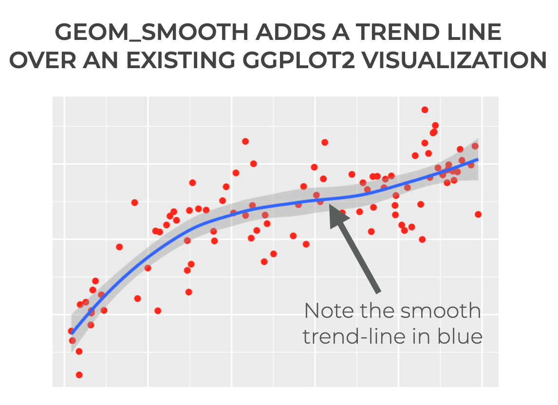
By default, the trend line that’s added is a LOESS smooth line. But there are a few options that allow you to change the nature of the line too. For example, you can add a straight “linear model” line.

The exact properties of the added line depend on the syntax.

That being said, let’s take a look at the syntax of the geom_smooth() function.

The syntax of Geom Smooth

Here, we’ll look at the syntax of geom_smooth.

A quick note

Note that to use geom_smooth, you need to have ggplot2 installed.

And, you need to have ggplot2 loaded into your environment.

You can do that with the code library(ggplot2), or the code library(tidyverse), which will load ggplot2, dplyr, and the other Tidyverse packages.

geom_smooth syntax

The syntax for using geom_smooth() is fairly simple.

We use this function in conjunction with an existing ggplot2 plot.

That means, you should already have a ggplot2 visualization created. Then, you can call geom_smooth() with the ‘+‘ sign.

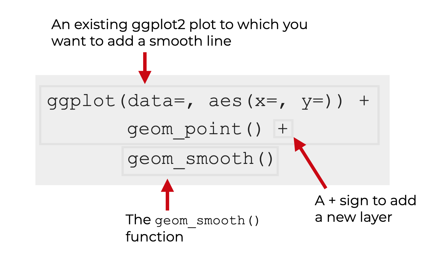
Additionally, there are some optional parameters that you can use inside the parenthesis to change the behavior of the function.

The parameters of geom_smooth

The geom_smooth function has a large number of optional parameters, but the most important that you should know are:

• mapping
• data
• span
• method
• formula
• se
• position
• na.rm
• orientation
• show.legend
• inherit.aes
• n
• fullrange
• level
• method.args

Let’s look at these one at a time.

data

The data parameter specifies the data associated with this smoothing line layer.

By default, geom_smooth will inherit the dataset that you specify with the top-line call to ggplot().

You can override that inherited data by supplying the name of a new dataframe to the data parameter. (You can provide objects besides dataframes, but they will be fortified to create a dataframe.)

mapping

This parameter enables you to specify a mapping from your data to the plot aesthetics.

By default, you don’t need to specify a mapping with this parameter, because typically, you’ll do so inside the ggplot() function and geom_smooth will inherit that mapping. (By default, the inherit.aes parameter is set to inherit.aes = False.)

If you set inherit.aes = True, then you’ll need to specify a mapping with this parameter.

method

The method parameter allows you to specify the smoothing function to use (i.e., the smoothing method).

There are several possible arguments to this parameter.

If you set this parameter to NULL, then it the function will use LOESS smoothing by default if there are fewer than 1000 observations, and mgcv::gam() if there are 1000+ observations.

You can also set it to the string values:

• "lm"
• "glm"
• "gam"
• "loess"

Or you can set it to an R stats function like:

• MASS::rlm
• mgcv::gam
• stats::lm
• stats::loess

formula

The formula allows you to specify an exact formula to use for the smoothing line.

For example, you could explicitly set “formula = y ~ x“.

se

The se parameter enables you to specify if you want a confidence interval around the smooth line.

By default, this is set to “se = True“. As you’ll see in the examples, this creates a dark-grey region around the smooth line. This dark grey area indicates the confidence interval (0.95 by default).

If you set “se = False“, it will remove the confidence interval.

position

The position parameter allows you to specify a position adjustment for the function.

na.rm

The na.rm parameter controls how the function handles missing values.

If you set “na.rm = False” then the function will remove missing values with a warning.

If you set “na.rm = True” then the function will remove missing values, but turn off the warning.

orientation

The orientation parameter controls the direction along which the smooth line is generated.

By default, this is set to “orientation = NA. This causes the function to determine the orientation automatically.

Alternatively, you can manually set the argument of this parameter to “x” or “y“.

show.legend

The show.legend parameter allows you to specify if the information about the the aesthetic mappings of the smoothing line layer.

By default, this is set to show.legend = NA which includes the information.

If you set show.legend = FALSE it will exclude the aesthetic mapping information from the legend.

inherit.aes

inherit.aes controls whether or not the geom_smooth layer will inherit aesthetic mappings from the top-line ggplot() function call.

By default, this is set to inherit.aes = TRUE.

If you set this to inherit.aes = FALSE, you will be able to manually override the default aesthetic mappings.

n

The n parameter controls the “number of points at which to evaluate” the smoothing function.

span

span specifies how much smoothing to use for the default LOESS smoothing function.

By default, this is set to span = 0.75.

As span increases, the smoothing line will become more smooth.

As span decreases, the smoothing line will become more rough and flexible.

Note that this parameter only applies when LOESS smoothing is used.

fullrange

fullrange controls whether the line should fit only the data, or the whole plot.

level

The level parameter controls the size of the confidence interval around the line.

This is set to level = .95 by default.

Final note on parameters

Keep in mind that most of these parameters are rarely used.

You’ll typically use only method, span, and possibly formula.

Examples of how to use geom_smooth

Now that we’ve looked at the syntax, let’s look at some examples of how to use geom smooth to add a smooth line or trend line to your data.

Examples:

• Add a LOESS smooth line
• Add a straight line “linear model”
• Change the smoothness/roughness of the smooth line

Setup code

Before you run the examples, you’ll need to run some setup code.

Specifically, you’ll need to:

• load the Tidyverse package
• create some sample data that we can visualize

Load tidyverse

First, you need to load the Tidyverse package.

library(tidyverse)

We’re mostly going to use ggplot2 for our visualizations, but we’ll also need the tibble() function in a moment to create a dataset. That being the case, it’s best to just load the whole tidyverse function instead of ggplot2 specifically.

Create data

Now, we’ll create a simple dataset that we can visualize.

Here, we’ll use the tibble() function to create a “tibble,” which is essentially just a fancy dataframe.

set.seed(55)
scatter_data <- tibble(x_var = runif(100, min = 0, max = 25)
                       ,y_var = log2(x_var) + rnorm(100)
             )

This dataset has two variables: x_var and y_var.

And let's quickly plot the data as a scatterplot with ggplot2:

ggplot(data = scatter_data, aes(x = x_var, y = y_var)) +
  geom_point(color = 'red')

OUT:

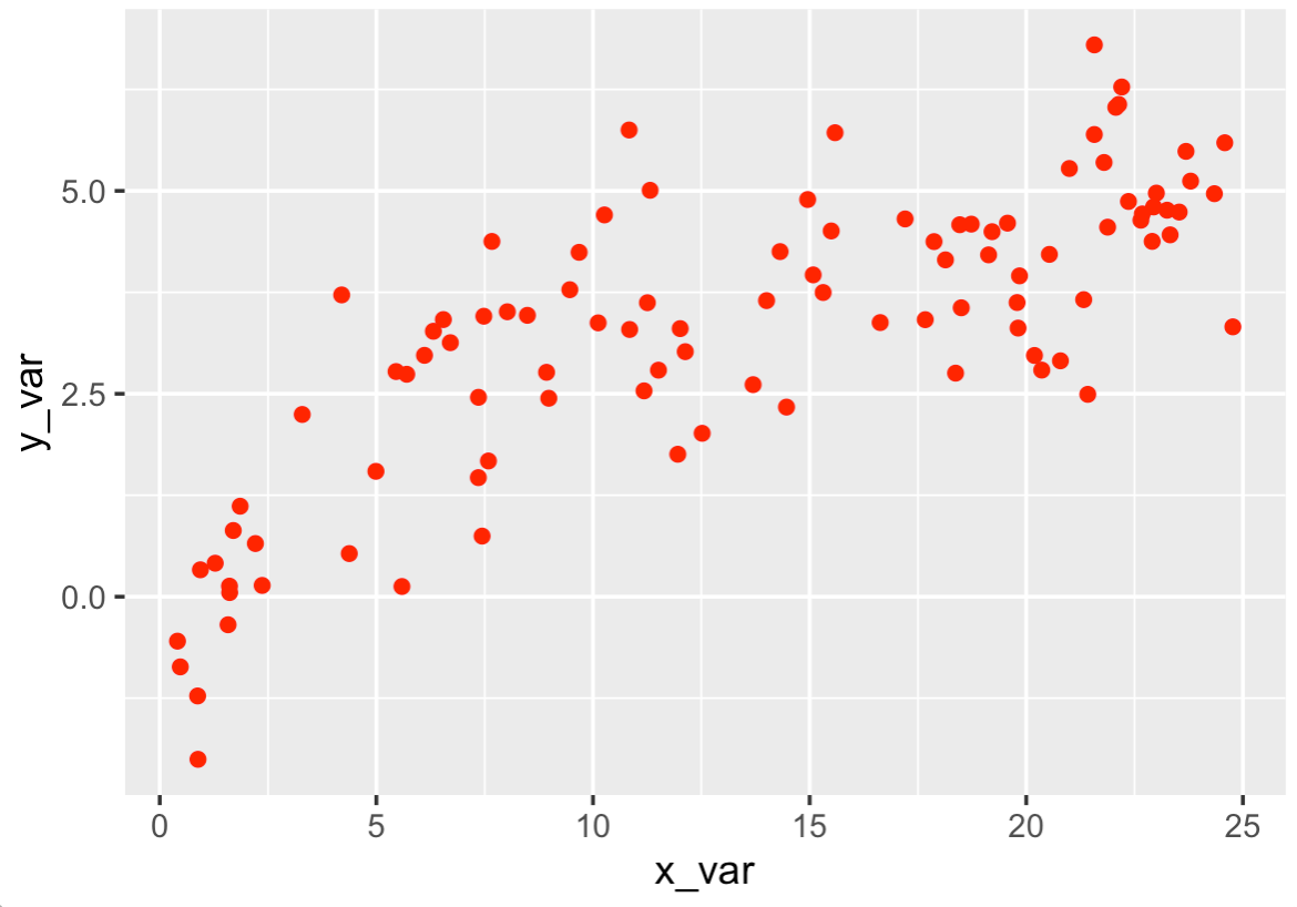
As you can see, there's a gentle curvilinear relationship between these two variables.

We'll use geom_smooth to visualize that relationship by adding a smooth line on top of this scatterplot.

EXAMPLE 1: Add a LOESS smooth line

First, we're going to add a LOESS smooth line over the scatterplot shown above.

Let's run the code, and then I'll explain.

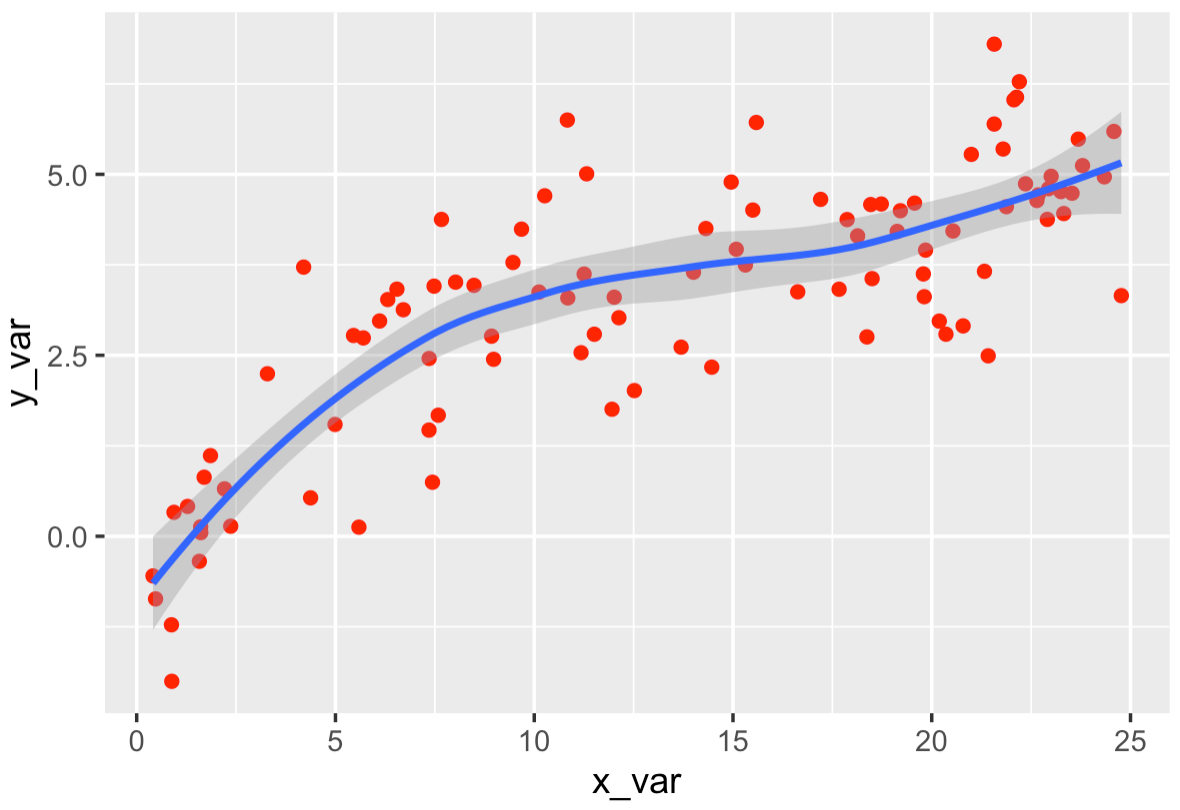
ggplot(data = scatter_data, aes(x = x_var, y = y_var)) +
  geom_point(color = 'red') +
  geom_smooth()

OUT:

Explanation

This is pretty straight forward.

Here, we created a scatterplot by calling ggplot() and geom_point().

To add a smooth line over it, we simply use the '+' symbol and then call geom_smooth().

Remember: ggplot2 allows you to build plots in layers. If you need to build a scatterplot with a smooth line over it, you literally write the code for the scatterplot, and then use the '+' symbol to add a new layer (the smooth line).

In this case, by default, the line is a LOESS (Locally Weighted Scatterplot Smoothing) line.

We can add different types of lines, however, which we'll do in the next example.

EXAMPLE 2: Add a straight line "linear model" with geom_smooth

Next, we're going to add a straight line over the scatterplot data.

Effectively, we'll use geom_smooth to create a simple linear model and plot that model over the data.

To do this, we'll set method = 'lm'.

Here's the code:

ggplot(data = scatter_data, aes(x = x_var, y = y_var)) +
  geom_point(color = 'red') +
  geom_smooth(method = 'lm')

And here's the output:

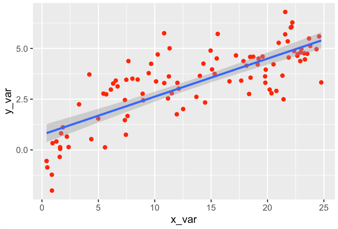
Explanation

This is pretty simple.

We have our scatterplot, and we're adding a trend line as a new layer with '+' and geom_smooth().

But in this case, we're adding a straight-line linear model instead of a LOESS line.

To do this, we simply set method = 'lm'. (If you haven't figured it out, 'lm' means "linear model.")

EXAMPLE 3: Change the smoothness/roughness of the smooth line

Finally, let's create a LOESS smooth line again, but let's create a rougher, more flexible line.

To do this, we'll use the span parameter.

ggplot(data = scatter_data, aes(x = x_var, y = y_var)) +
  geom_point(color = 'red') +
  geom_smooth(span = .2)

OUT:

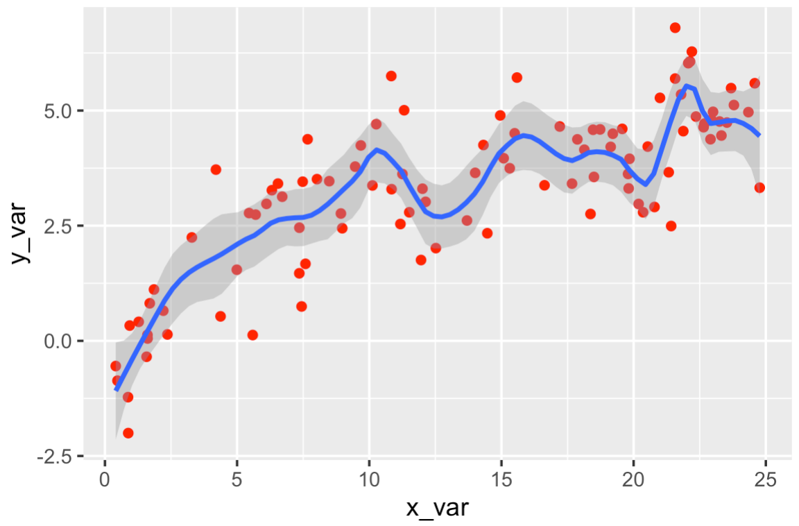
Explanation

Here, to create the LOESS line, we're calling geom smooth, much like we did in example 1.

The major difference here is that we're using the span parameter to change the smoothness of the line.

Specifically, we decreased the span to .2 (the default is .75).

As span decreases, the line will become rougher and as span increases, the line will become smoother.

Keep in mind that it may take some trial-and-error to find the ideal value for span.

Not also that in this case, lowering the span may actually be bad. It's causing the line to follow some of the noise in the data, instead of the more general underlying pattern.

You need to take care when you use this parameter.

Frequently asked questions about KEYWORD

Now that you've learned about geom_smooth and seen some examples, let's review some frequently asked questions.

Frequently asked questions:

• What's the difference between geom_smooth and stat_smooth?

Question 1: What's the difference between geom_smooth and stat_smooth?

Effectively, there is no difference. They are almost identical.

The only difference is that stat_smooth allows you to make a plot with a "non standard geom."

Leave your other questions in the comments below

Do you have other questions about geom_smooth?

Leave your questions in the comments section below.

For more data science tutorials, sign up for our email list

This tutorial showed you how to use geom_smooth to add a trend line to your ggplot2 plots.

But if you want to master data science and data visualization in R, there's a lot more to learn.

That said, to learn more about data science with R, then sign up for our email list.

When you sign up, you’ll get free tutorials on:

• R
• ggplot2
• dplyr
• machine learning
• ... as well as tutorials about data science with Python

If you're interested in learning more data science, then enter your best email below: