There’s sort of an open secret in the data science world:
As a data professional, you’ll spend a huge amount of time doing data preparation.
Cleaning, joining, reshaping, aggregating …
These tasks make up a huge amount of your data work. Many data professionals say as much as 80%.
You Need to Master Data Manipulation
Because data manipulation is so important, it’s something you need to focus on relentlessly.
This is particularly true in the beginning. When you’re first starting to learn data science, you should really focus on two core skills: data manipulation and data visualization.
Because data manipulation is so important, I want to give you a crash course in how to do data manipulation in R.
dplyr: Essential Data Manipulation Tools for R
If you’re doing data science in the R programming language, that means that you should be using dplyr.
If you’re not really familiar with it, dplyr is a data manipulation package for R.
Moreover, dplyr is one of the modules of the so-called “Tidyverse.” The Tidyverse is a collection of R packages for doing data science, which includes dplyr, ggplot2, tidyr, forcats, and several others.
dplyr focusses on data manipulation
Although the packages of the Tidyverse all deal with data science in one way or another, dplyr focusses on data manipulation.
One of the brilliant things about dplyr though is the simplicity.
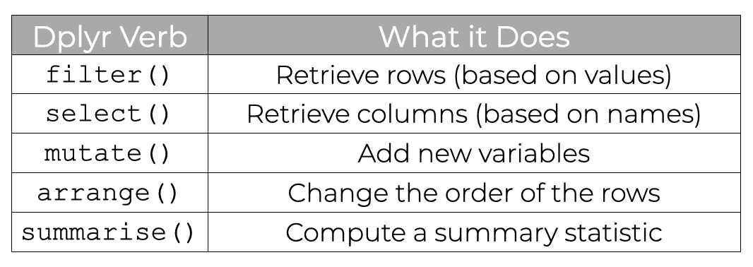
At its core, dplyr really only has 5 major functions, which we sometimes call “verbs.”
Each of these dplyr verbs does one thing.
Each verb is named in a way that is extremely easy to remember.
And all of the verbs can be combined together to perform more complex data manipulations (which I’ll explain in the section about dplyr “chains”).
Let’s talk about these data manipulation “verbs.”
The 5 Dplyr Verbs
Dplyr has 5 primary verbs.
These verbs are essentially commands, and each one does one thing.
I’ll show you examples of these in the examples section, but first, let’s quickly look at the syntax.
Dplyr Syntax
All of the primary dplyr functions (i.e., verbs) share a similar syntax.
You can use them like this:
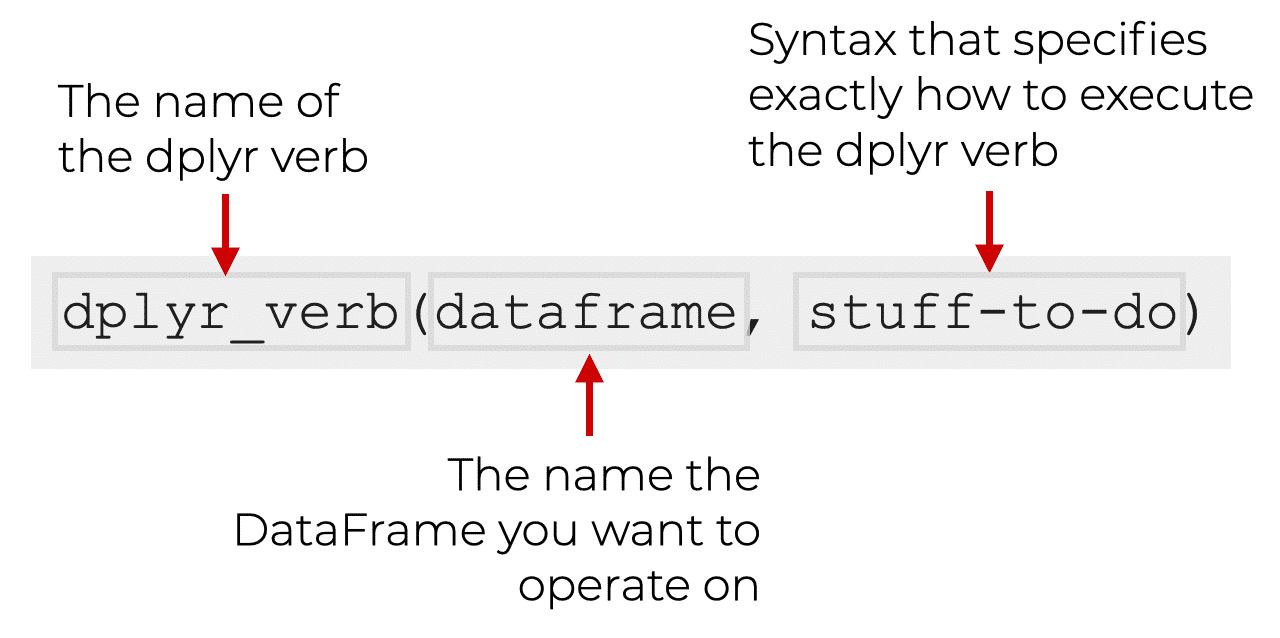
Essentially, you call the function. Inside the parenthesis, the first argument (i.e., the first input) is the name of the dataframe you want to operate on.
Then, after that, there is some syntax that specifies exactly what to do with the dplyr function. This will be different for every dplyr function, so look at the upcoming examples to see exactly how each one works.
Keep in mind though, that this is the normal syntax for using the dplyr verbs. There’s also another way to use the dplyr verbs using “pipes”. I’ll explain that in the section on dplyr pipes.
Ok, now that you’ve learned about the general syntax of the dplyr functions, let’s look at some examples.
Dplyr Function Examples
In this section, we’ll take a look at some simple, yet concrete examples of each of the 5 dplyr verbs.
To be clear: these will not be comprehensive examples. They won’t show you everything that dplyr can do.
But they will get you started by show you most of the basic functionality.
Run this code first
Before you look at the following examples, you’ll need to run some code first.
Open up R Studio (or whatever IDE you’re using) and run the following:
library(tidyverse)
library(dplyr)
data(starwars)
This will load the tidyverse collection of packages, and will also retrieve our dataset.
Here, we’ll be working with the starwars dataset.
Ok. Now that you’ve done that, let’s look at the verbs.
FILTER()
First, we have filter.
The filter() verb selects rows of data based on value.
Another way of saying this is that filter selects rows based on logical criteria that involve values.
That might sound complicated, but it’s actually really simple once you understand.
Let’s take a look so I can explain.
Let’s say that we want to identify Star Wars characters who are droids.
We can do that with the filter technique.
filter(starwars, species == 'Droid')
OUT:
 name  height  mass hair_color skin_color eye_color birth_year gender homeworld species
1 C-3PO    167    75 NA         gold       yellow           112 NA     Tatooine  Droid
2 R2-D2     96    32 NA         white, bl… red               33 NA     Naboo     Droid
3 R5-D4     97    32 NA         white, red red               NA NA     Tatooine  Droid
4 IG-88    200   140 none       metal      red               15 none   NA        Droid
5 BB8       NA    NA none       none       black             NA none   NA        Droid
Notice that the output is the rows for droid characters.
Explanation
Here, we’ve used the dplyr filter function on the starwars dataset.
After calling the function, the first argument is the name of the dataframe.
The second argument is a logical condition that specifies which rows we want to retrieve. Look at the code species == 'Droid'. Remember that species is one of the variables. 'Droid' is one of the categories in that variable.
So essentially, we’re subsetting our data based on a logical condition.
If the condition species == 'Droid' is true for a particular row, then it is returned in the subset. If that condition is false, it is not returned.
Keep in mind that this is just one example. You can also subset on multiple variables, numeric variables, and more. There are a variety of types of logical conditions that we can use to subset our data with filter().
For more insight into how to use filter(), check out our tutorial on the dplyr filter function.
SELECT()
Next, let’s take a look at the select() verb.
Select retrieves columns.
So whereas filter retrieves rows, select retrieves columns. (Remember: in dplyr, every function essentially does only one thing).
When we use select, we retrieve the columns based on name.
Here’s an example.
Let’s say that we want to retrieve only 3 columns: name, species, and homeworld.
This is extremely easy to do with select().
We simply call the name of the function, and inside the parenthesis, we provide the name of the dataframe, and the name of each column we want to return.
select(starwars, name, species, homeworld)
OUT:
   name               species homeworld
 1 Luke Skywalker     Human   Tatooine
 2 C-3PO              Droid   Tatooine
 3 R2-D2              Droid   Naboo
 4 Darth Vader        Human   Tatooine
 5 Leia Organa        Human   Alderaan
 6 Owen Lars          Human   Tatooine
 7 Beru Whitesun lars Human   Tatooine
 8 R5-D4              Droid   Tatooine
 9 Biggs Darklighter  Human   Tatooine
10 Obi-Wan Kenobi     Human   Stewjon
# … with 77 more rows
Explanation
Here, the output consists of all of the rows of data, but only 3 columns: name, species, and homeworld.
Notice syntactically, how simple it is. We simply call the function, provide the name of the dataframe and then provide the names of the columns we want to return. We don’t even need to enclose the names of the columns in quotations. Just provide the name of each column you want to return, separated by commas. Everything is clean and simple.
Also, notice something about the output. The columns are returned in exactly the order that we list them as the arguments to the function.
MUTATE()
The mutate function adds new variables to a dataframe.
Again, like the other dplyr functions, mutate is extremely easy to use.
First, we call the name of the function.
Then inside the parenthesis, we first provide the name of the dataframe.
And after that, we provide an expression that defines a new variable name, and how to compute it. (We call this a “name/value pair.”)
Let’s take a look.
The mass variable in the dataframe is the mass of the character, in kilograms.
But let’s say that we want to compute the weight, in pounds. We can do that with mutate.
Here, we’re going to use mutate to create a new variable called weight_lbs.
mutate(starwars, weight_lbs = mass * 2.2)
OUT:
name height mass hair_color skin_color eye_color birth_year gender homeworld species weight_lbs1 Luke Skywa… 172 77 blond fair blue 19 male Tatooine Human 169. 2 C-3PO 167 75 NA gold yellow 112 NA Tatooine Droid 165 3 R2-D2 96 32 NA white, bl… red 33 NA Naboo Droid 70.4 4 Darth Vader 202 136 none white yellow 41.9 male Tatooine Human 299. 5 Leia Organa 150 49 brown light brown 19 female Alderaan Human 108. 6 Owen Lars 178 120 brown, grey light blue 52 male Tatooine Human 264 7 Beru White… 165 75 brown light blue 47 female Tatooine Human 165 8 R5-D4 97 32 NA white, red red NA NA Tatooine Droid 70.4 9 Biggs Dark… 183 84 black light brown 24 male Tatooine Human 185. 10 Obi-Wan Ke… 182 77 auburn, wh… fair blue-gray 57 male Stewjon Human 169. # … with 77 more rows
In the output, the new variable is all the way at the right hand side, so you might need to scroll to see it.
(Note: I removed a few columns so we could view the new column easier.)
Explanation
Here, we used the mutate() function to create a new variable called weight_lbs. You can see this new variable at the far right hand side of the output.
How did we do it?
We simply called the mutate function like this:
mutate(starwars, weight_lbs = mass * 2.2)
Inside of the parenthesis, we’re specifying that we want to operate on the starwars dataframe.
And specifically, we’re specifying that we want to create a new variable called weight_lbs that will be equal to the value in the mass variable, times 2.2.
That’s it. Adding a variable with mutate is just that simple. You can even add multiple new variables by specifying additional name-value pairs, separated by commas.
Having said that, in spite of the simplicity here, using mutate can be more complex. This is particularly true when we’re creating a variable that’s based on some complex computation.
That being said, this example should get you started, but for more information, check out our tutorial on the dplyr mutate verb.
ARRANGE()
Now, let’s look at the arrange function.
The arrange function sorts a dataframe.
Like the other dplyr functions, arrange is very easy to use.
We simply call the name of the function. Inside the parenthesis, we specify the dataframe we want to operate on, and then the variable or variables that we want to sort by.
Let’s take a look. Here, we’ll sort by height.
arrange(starwars, height)
OUT:
   name  height  mass hair_color skin_color eye_color birth_year gender homeworld species
 1 Yoda      66    17 white      green      brown            896 male   NA        Yoda …
 2 Ratt…     79    15 none       grey, blue unknown           NA male   Aleen Mi… Aleena
 3 Wick…     88    20 brown      brown      brown              8 male   Endor     Ewok
 4 Dud …     94    45 none       blue, grey yellow            NA male   Vulpter   Vulpte…
 5 R2-D2     96    32 NA         white, bl… red               33 NA     Naboo     Droid
 6 R4-P…     96    NA none       silver, r… red, blue         NA female NA        NA
 7 R5-D4     97    32 NA         white, red red               NA NA     Tatooine  Droid
 8 Sebu…    112    40 none       grey, red  orange            NA male   Malastare Dug
 9 Gasg…    122    NA none       white, bl… black             NA male   Troiken   Xexto
10 Watto    137    NA black      blue, grey yellow            NA male   Toydaria  Toydar…
# … with 77 more rows
Explanation
Here, we’re sorting the data by height.
By default, arrange() sorts the data in ascending order (notice Yoda at the top).
We can actually sort in descending order by using the desc() helper function:
arrange(starwars, desc(height))
Keep in mind that this is a fairly simple example. It is possible to sort in more complex ways, such as multiple variables, etc.
SUMMARIZE()
Finally, let’s look at the summarize() function.
Summarize summarizes your data.
For example, if you need to calculate things like a mean, median, count, sum, etc … you can do this with summarize().
Let’s look at an example.
Here, we’ll calculate the average height.
summarise(starwars, mean(height, na.rm = TRUE))
OUT:
  `mean(height, na.rm = TRUE)`
                          174.
Explanation
Ok, this one is a little more complicated, but still pretty easy.
The summarize function summarizes your data.
Here, we’re calculating the average height. To do this, we need to use the mean() function.
So we’re calling summarize().
Inside the parenthesis, the first argument is the name of the dataframe.
The second argument is where we call the mean function. Here, we’re using height as the input to mean(), and we’re setting na.rm = TRUE to deal with missing values.
Compared to the other dplyr verbs, summarize can be a little more complicated. We typically need to use summarization functions (like mean, median and others) to get it to work properly. And there are some other options that enable use to change the output, like providing a name for the summarized variable.
Still, the summarize function is fairly easy to use.
Remember: dplyr verbs create new dataframes
One quick note about all of these dplyr functions.
All of these functions create new dataframes.
What that means is that these functions do not directly change the original dataframe.
Typically, the output is sent to the console in R studio, and is unsaved.
If you want to save the output, assign it to a variable
If you want to save the output, you need to pass the output to a variable name using the assignment operator.
Here is an example:
starwars_droids <- filter(starwars, species == 'Droid')
Here, we're subsetting retrieving the droids from the data using the filter verb, with species == 'Droid'.
But notice that we're using the assignment operator (<-)to assign the output to the variable name starwars_droids. This keeps the original dataframe intact, and saves the new subsetted data to a new variable name.
Alternatively, we could overwrite and update the original dataset, also using the assignment operator:
starwars <- filter(starwars, species == 'Droid')
Be careful with this!
This will overwrite the original starwars dataframe with the smaller subset of only droids!
Again, be careful when you're assigning the output to the original variable name. Make sure that your code is working properly, and that you're sure you want to overwrite the original.
How to Use Dplyr Pipes
Now that you've learned about the 5 primary dplyr verbs, let's quickly talk about dplyr pipes.
The %>% Operator
In dplyr and the larger Tidyverse (i.e., ggplot2, tidyr, etc) we can use a special operator to chain together multiple commands.
This operator, %>% is typically called the pipe operator (although I think that the term "chaining" makes more sense, and you might see me refer to dplyr "chains").
We can use this operator to combine together multiple dplyr functions in a chain. This enables us to perform much more complicated data manipulations.
Dplyr Pipe Syntax
Let's quickly look at the syntax for how we use the dplyr pipe.
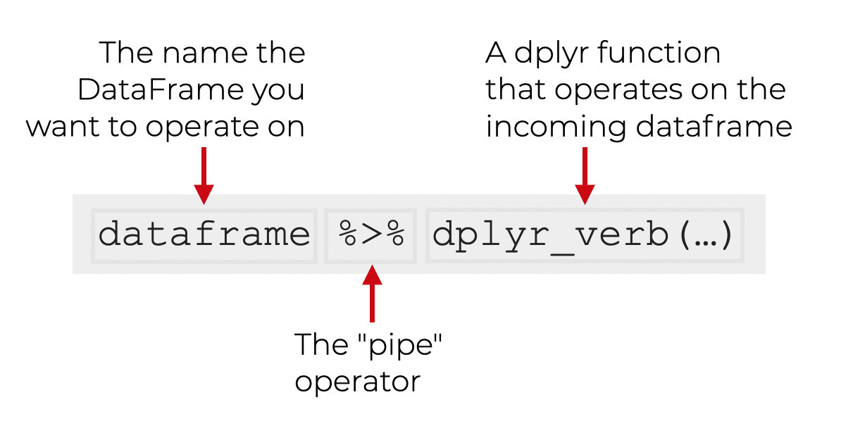
Notice that when we use a dplyr pipe, the syntax is sort of turned inside-out.
Typically, when we use this technique, the syntax starts with the name of the dataframe.
Then we use the pipe operator to "pipe" the dataframe as an input into the dplyr function. (And inside of the dplyr function, the rest of the syntax will work as normal.)
This might sound complicated, but it's really simple once you see it, so let's look at an example.
A Simple Example of a Dplyr Chain
Let's start by looking at a simple example.
Here, we're going to redo the example from the section on filter.
Previously, we created a subset of data where species == 'Droid'.
The code looked like this:
filter(starwars, species == 'Droid')
Now, we're going to rebuild that code and use a dplyr pipe:
starwars %>% filter(species == 'Droid')
Both examples will produce the exact same output.
The only difference between these is that the second uses a dplyr pipe.
Multi-step dplyr chains
So why would we do this?
What's the advantage to using the pipe operator like this?
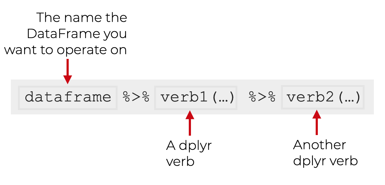
The advantage is that we can use multiple pipes in a row, such that the output of one dplyr function becomes the input of another dplyr function.
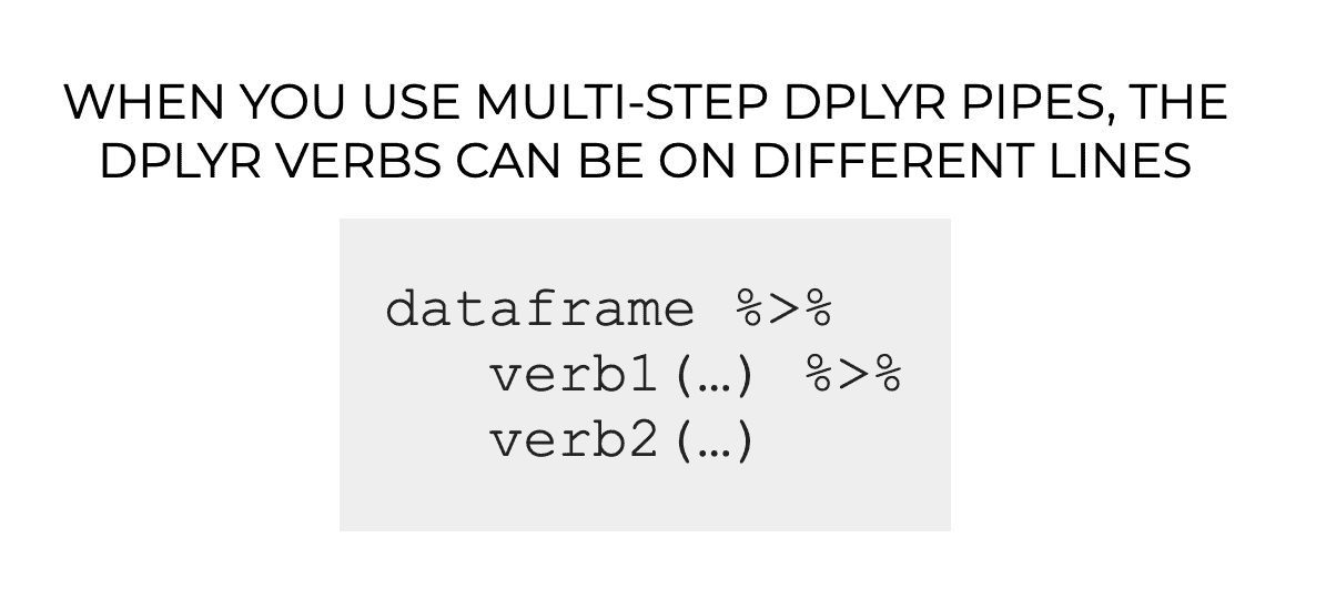
Keep in mind that you can also put the dplyr verbs on different lines ... they don't all need to be on the same line.
This technique is extremely powerful.
Dplyr chaining syntax enables you to create multi-step data manipulations that modify your data in complex ways.
This is really what makes dplyr so much better than almost any other data wrangling toolkit available.
An Example of a Multi-step Dplyr Chain
Let's take a look at an example of a multi-step dplyr chain.
We're going to get some basic stats for the characters born on Tatooine, and sort them by age.
To do this, we'll start with the starwars dataframe, then we'll use filter to subset down to the characters that were from Tatooine. Then we'll use select to retrieve only a few specific columns, and we'll use arrange to sort the data.
starwars %>%
  filter(homeworld == 'Tatooine') %>%
  select(name, species, height, mass, birth_year) %>%
  arrange(desc(birth_year))
OUT:
   name               species height  mass birth_year
 1 C-3PO              Droid      167    75      112
 2 Cliegg Lars        Human      183    NA       82
 3 Shmi Skywalker     Human      163    NA       72
 4 Owen Lars          Human      178   120       52
 5 Beru Whitesun lars Human      165    75       47
 6 Darth Vader        Human      202   136       41.9
 7 Anakin Skywalker   Human      188    84       41.9
 8 Biggs Darklighter  Human      183    84       24
 9 Luke Skywalker     Human      172    77       19
10 R5-D4              Droid       97    32       NA
The output gives us a sorted subset of a few important columns.
But notice the syntax.
We combined multiple dplyr functions together using the %>% operator.
When we do this, we start with the dataframe and "pipe" it as an input to the first dplyr function (filter, in this case).
Then we can take the output of any given dplyr function and use the %>% operator to pipe the output of one function into the next one.
Using %>%, the output dataframe of one function becomes the input dataframe to the next.
Read the pipe operator as 'then'
One additional comment about the syntax.
One good practice, is when you're reading code that uses the pipe operator, you should read it as "then."
Let's take a look at that chaining code again, but here, I'll add some comments to show how to read it.
starwars %>%                                            # Start with the starwars dataset
  filter(homeworld == 'Tatooine') %>%                   # THEN retrieve the rows where homeworld == 'Tatooine'
  select(name, species, height, mass, birth_year) %>%   # THEN retrieve the name, species, height, mass, and birth_year variables
  arrange(desc(birth_year))                             # THEN sort the data in descending order, by birth year
At every step, we can read the code like a series of procedures.
Do something .... then do something else .... then do another thing ... etc.
One of the reasons that this technique is so powerful is that it makes your code so f*cking easy to read.
Part of the power is the combinatorial nature of the technique (which I'll mention in a moment), but a huge part of the benefit is that you can read your code in this top-to-bottom, serial fashion.
Perform complex data manipulation with dplyr chains
What's great about dplyr is that you have a set of simple, easy-to-use functions that can be combined in complex ways using pipes.
This makes your code easy to read, easy to write, and easy to debug.
But moreover, the process of performing data manipulation just becomes a problem of combining little building blocks ... almost like snapping together little LEGO blocks to create a larger structure.
It's brilliant, powerful, and frankly, a joy to use.
Rapid Data Exploration With Dplyr and ggplot2
Ok. One last thing.
You can use dplyr in combination with ggplot2 (and other functions of the Tidyverse) to do rapid data analysis and exploration.
Again, this is why the Tidyverse system is so powerful. You can combine together multiple simple tools to perform complex operations. Everything snaps together.
Example: barplot, dplyr + ggplot2
Here, we're going to subset our data and then create a bar chart.
Here, we're going to filter the data down to the human characters (and we'll remove the records where height equals NA).
After filtering the data, we'll use ggplot2 to plot the data.
Notice as you read the code, that we're using dplyr pipes to combine together a couple of dplyr functions. Then we're piping the output of those dplyr subsetting functions into ggplot2!
They work together seamlessly.
starwars %>%
  select(name, gender, height, species) %>%
  filter(species == 'Human') %>%
  filter(!is.na(height)) %>%
  ggplot(aes(y = fct_reorder(name, height), x = height, fill = gender) ) +
    geom_bar(stat = 'identity') +
    scale_fill_manual(values = c('maroon', 'navy'))
OUT:
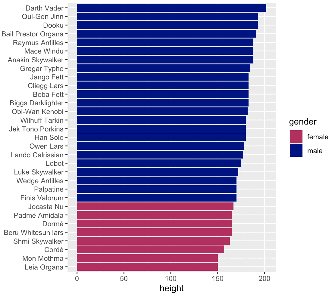
This is not terribly complicated, but it shows some of the power of the dplyr/ggplot2/Tidyverse system.
Here, we're combining together a couple of dplyr functions to subset the data (we could use even more dplyr functions, if we wanted to perform other data manipulations).
Then we're taking the output of the final filter() call and piping it into ggplot2 to visualize the data and create a bar chart.
To be clear: this might seem a little complex if you're unfamiliar with these functions. But if you break it down, there are only 6 or 7 techniques (i.e., Tidyverse functions) that we're using here. We're just taking relatively simple tools and combining them together.
Moreover, once you master these tools, you can do much, much more.
Dplyr is One of the Foundations of Data Science in R
Data manipulation is a foundational skill.
If you want to master data science, you must become highly proficient in data manipulation.
And if you choose to use R, I recommend that you use dplyr.
There are other data manipulation tools for R, but dplyr is easy to learn, easy to use, and extremely powerful.
Once you master the essential techniques of dplyr, you'll wish you had learned it a lot sooner.
Enroll in our course to master dplyr
The dplyr examples here are pretty simple and easy to understand.
But other parts of dplyr and the Tidyverse can be a lot more complicated.
If you're serious about learning dplyr and data science in R, you should consider joining our premium course called Starting Data Science with R.
Starting Data Science will teach you all of the essentials you need to do data science in R, including:
- How to manipulate your data with dplyr
- How to visualize your data with ggplot2
- Tidyverse helper tools, like tidyr and forcats
- How to analyze your data with ggplot2 + dplyr
- and more ...
Moreover, it will help you completely master the syntax within a few weeks. We'll show you a practice system that will enable you to memorize all of the R syntax you learn. If you have trouble remembering R syntax, this is the course you've been looking for.
We're reopening Starting Data Science tomorrow, January 5, 2021.
You can find out more here:
Me gustaría mucho apreder a usar dplyr y tidyverse.