In this tutorial, I’ll show you how to use the loc method to select data from a Pandas dataframe.
If you’re new to Pandas and new to data science in Python, I recommend that you read the whole tutorial. There are some little details that can be easy to miss, so you’ll learn more if you read the whole damn thing.
But, I get it. You might be in a hurry.
Fair enough.
Here are a few links to the important sections:
- A quick refresher on Pandas
- Pandas DataFrame basics
- The syntax of Pandas loc
- Examples: how to use the Pandas loc method
Again though, I recommend that you slow down and learn step by step. That’s the best way to rapidly master data science.
Ok. Quickly, I’m going to give you an overview of the Pandas module. The specifics about loc[] will follow just afterwards.
A quick refresher on Pandas
To understand the Pandas loc method, you need to know a little bit about Pandas and a little bit about DataFrames.
What is Pandas?
Pandas is a data manipulation toolkit in Python
Pandas is a module for data manipulation in the Python programming language.
At a high level, Pandas exclusively deals with data manipulation (AKA, data wrangling). That means that Pandas focuses on creating, organizing, and cleaning datasets in Python.
However, Pandas is a little more specific.
Pandas focuses on DataFrames. This is important to know, because the loc technique requires you to understand DataFrames and how they operate.
That being the case, let’s quickly review Pandas DataFrames.
Pandas DataFrames basics
A Pandas DataFrame is essentially a 2-dimensional row-and-column data structure for Python.
This row-and-column format makes a Pandas DataFrame similar to an Excel spreadsheet.
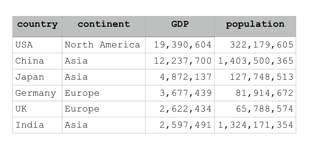
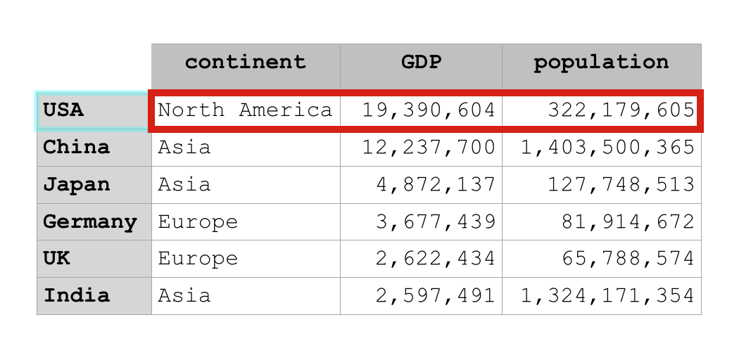
Notice in the example image above, there are multiple rows and multiple columns. Also notice that different columns can contain different data types. A column like ‘continent‘ contains string data (i.e., character data) but a different column like ‘population‘ contains numeric data. Again, different columns can contain different data types.
But, within a column, all of the data must have the same data type. So for example, all of the data in the ‘population‘ column is integer data.
Pandas dataframes have indexes for the rows and columns
Pandas DataFrames have another important feature: the rows and columns have associated index values.
Take a look. Every row has an associated number, starting with 0. Every column also has an associated number.
These numbers that identify specific rows or columns are called indexes.
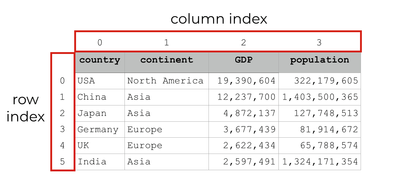
Keep in mind that all Pandas DataFrames have these integer indexes by default.
Integer indexes are useful because you can use these row numbers and column numbers to select data and generate subsets. In fact, that’s what you can do with the Pands iloc[] method. Pandas iloc enables you to select data from a DataFrame by numeric index.
But you can also select data in a Pandas DataFrames by label. That’s really important for understanding loc[], so let’s discuss row and column labels in Pandas DataFrames.
Pandas dataframes can also have ‘labels’ for the rows and columns
In addition to having integer index values, DataFrame rows and columns can also have labels.
Unlike the integer indexes, these labels do not exist on the DataFrame by default. You need to define them. (I’ll show you how in a moment.)
When you set them up, the row and column labels look something like this:
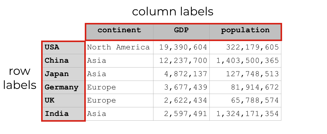
Importantly, if you set the labels up right, you can use these labels to subset your data.
And that’s exactly what you can do with the Pandas loc method.
The loc method: how to select data from a dataframe
So now that we’ve discussed some of the preliminary details of DataFrames in Python, let’s really talk about the Pandas loc method.
The Pandas loc method enables you to select data from a Pandas DataFrame by label.
It allows you to “locate” data in a DataFrame.
That’s where we get the name loc[]. We use it to locate data.
It’s slightly different from the iloc[] method, so let me quickly explain that.
How is Pandas loc different from iloc?
This is very straightforward.
The loc method locates data by label.
The iloc method locates data by integer index.
I’m really not going to explain iloc here, so if you want to know more about it, I suggest that you read our Pandas iloc tutorial.
The syntax of the Pandas loc method
Now that you have a good understanding of DataFrame structure, DataFrame indexes, and DataFrame labels, lets get into the details of the loc method.
Here, I want to explain the syntax of Pandas loc.
How does it work?
If you’re familiar with calling methods in Python, this should be very familiar.
Essentially, you’re going to use “dot notation” to call loc[] after specifying a Pandas Dataframe.
So first, you’ll specify a Pandas DataFrame object.
Then, you’ll type a dot (“.“) ….
… followed by the method name, loc[].
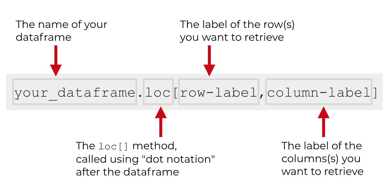
Inside of the loc[] method, you need to specify the labels of the rows or columns that you want to retrieve.
It’s important to understand that you can specify a single row or column. Or you can also specify a range of rows or columns. Specifying ranges is called “slicing,” and it’s an important tool for subsetting data in Python. I’ll explain more about slicing later in the examples section of this tutorial.
An important note about the ‘column’ label
There’s one important note about the ‘column’ label.
If you don’t provide a column label, loc will retrieve all columns by default.
Essentially, it’s optional to provide the column label. If you leave it out, loc[] will get all of the columns.
Examples of Pandas loc
Ok. Now that I’ve explained the syntax at a high level, let’s take a look at some concrete examples.
Here’s what I will show you:
- row selection with loc
- column selection with loc
- retrieve specific cells with loc
- retrieve ranges of rows and columns (i.e., slicing)
- get specific subsets of cells
In this examples section, we’re going to focus on simple examples. This is important. When you’re learning, it’s very helpful to work with simple, clear examples. Don’t try to get fancy too early on. Learn the technique with simple examples and then move on to more complex examples later.
Before we actually get into the examples though, we have two things we need to do. We need to import Pandas and we need to create a simple Pandas DataFrame that we can work with.
Import modules
First, we’ll just import Pandas.
We can do this with the following code.
#===============
# IMPORT MODULES
#===============
import pandas as pd
Note that we’re importing Pandas with the alias pd. This makes it possible to refer to Pandas as pd in our code, which simplifies things a little.
Create DataFrame
Next, we’re going to use the pd.DataFrame function to create a Pandas DataFrame.
There’s actually three steps to this. We need to first create a Python dictionary of data. Then we need to apply the pd.DataFrame function to the dictionary in order to create a dataframe. Finally, we’ll specify the row and column labels.
Here’s the step where we create the Python dictionary:
#==========================
# CREATE DICTIONARY OF DATA
#==========================
country_data_dict = {
    'country':['USA', 'China', 'Japan', 'Germany', 'UK', 'India']
    ,'continent':['North America','Asia','Asia','Europe','Europe','Asia']
    ,'GDP':[19390604, 12237700, 4872137, 3677439, 2622434, 2597491]
    ,'population':[322179605, 1403500365, 127748513, 81914672, 65788574, 1324171354]
}
Next, we’ll create our DataFrame from the dictionary:
#=================================
# CREATE DATAFRAME FROM DICTIONARY
#=================================

country_data_df = pd.DataFrame(country_data_dict)
Finally, we need to set the row labels. By default, the row labels will just be the integer index value starting from 0.
Here though, we’re going to manually change the row labels.
Specifically, we’re going to use the values of one of our existing columns, country, as the row labels.
To do this, we’ll use the set_index() method from Pandas:
country_data_df = country_data_df.set_index('country')
Notice that we need to store the output of set_index() back in the DataFrame, country_data_df by using the equal sign. This is because set_index() creates a new object by default; it doesn’t modify the DataFrame in place.
Quickly, let’s examine the data with a print statement:
print(country_data_df)
             continent       GDP  population
country
USA      North America  19390604   322179605
China             Asia  12237700  1403500365
Japan             Asia   4872137   127748513
Germany         Europe   3677439    81914672
UK              Europe   2622434    65788574
India             Asia   2597491  1324171354
You can see the row-and-column structure of the data. There are 3 columns: continent, GDP, and population. Notice that the “country” column is set aside off to the left. That’s because the country column has actually become the row index (the labels) of the rows.
Visually, we can represent the data like this:
Essentially, we have a Pandas DataFrame that has row labels and column labels. We’ll be able to use these row and column labels to create subsets.
With that in mind, let’s move on to the examples.
Select a single row with the Pandas loc method
First, I’m going to show you how to select a single row using loc.
Example: select data for USA
Here, we’re going to select all of the data for the row USA.
To do this, we’ll simply call the loc[] method after the dataframe:
country_data_df.loc['USA']
Which produces the following output:
continent     North America
GDP                19390604
population        322179605
Name: USA, dtype: object
This is fairly straightforward, but let me explain.
We’re using the loc[] method to select a single row of data by the row label. The row label for the first row is ‘USA,’ so we’re using the code country_data_df.loc['USA'] to pull back everything associated with that row.
Notice that using loc[] in this way returns the values for all of the columns for that row. It tells us the continent of USA (‘North America‘), the GDP of USA (19390604), and the population of the row for USA (322179605).
The loc method returns all of the data for the row with the label that we specify.
Example: select data for India
Here’s another example.
Here, we’re going to select all of the data for India. In other words, we’re going to select the data for the row with the label India.
Once again, we’ll simply use the name of the row label inside of the loc[] method:
country_data_df.loc['India']
Which produces the following output:
continent           Asia
GDP              2597491
population    1324171354
Name: India, dtype: object
As you can see, the code country_data_df.loc['India'] returns all of the data for the ‘India‘ row.
Now that I’ve shown you one way to select data for a single row, I’m going to show you an alternate syntax.
Select a single row (alternate syntax)
There’s actually another way to select a single row with the loc method.
It’s a little more complicated, but it’s relevant for retrieving “slices” of data, which I’ll show you later in this tutorial.
Here, we’re going to call the loc[] method using dot notation, just like we did before.
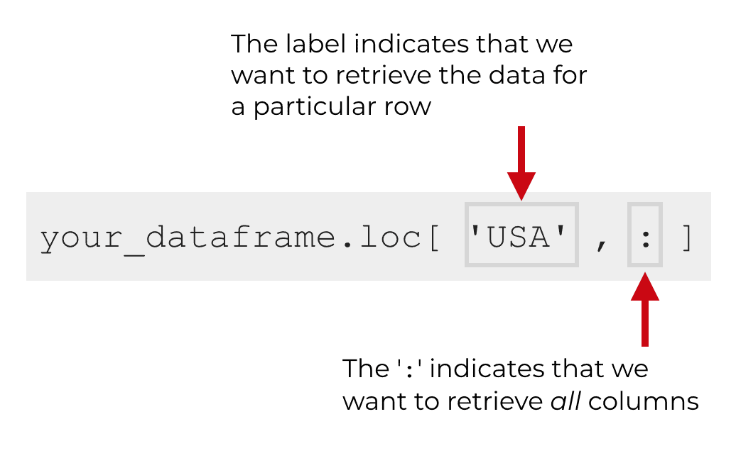
Inside of the loc[] method, the first argument will be the label associated with the row we want to return. Here, we’re going to retrieve the data for USA, so the first argument inside of the brackets will be ‘USA.’
After that though, the code will be a little different. After the row label that we want to return, we have a comma, followed by a colon (‘:‘).
The full line of code looks like this:
country_data_df.loc['USA',:]
Which produces the following:
continent     North America
GDP                19390604
population        322179605
Name: USA, dtype: object
Once again, this code has pulled back the row of data associated with the label ‘USA.’
The output of this code is effectively the same as the code country_data_df.loc['USA']. The difference is that we’re using a colon inside of the brackets now (i.e., country_data_df.loc['USA',:]).
Why?
Remember from earlier in this tutorial when I explained the syntax: when we use the Pandas loc method to retrieve data, we can refer to a row label and a column label inside of the brackets.
In the code country_data_df.loc['USA',:], ‘USA‘ is the row label and the colon is functioning as the column label.
But instead of referring to a specific column, the colon basically tells Pandas to retrieve all columns.
The output though is basically the row associated with the row label ‘USA‘:
Keep this syntax in mind … it will be relevant when we start working with slices of data.
Ok. Now that you’ve learned how to select a single row of data from a Python dataframe, let’s look at how to select a single column of data.
Select columns with Pandas loc
Selecting a column from a Python DataFrame is fairly simple syntactically. It’s very similar to the syntax for selecting a row.
The major difference is how we specify the row and column labels inside of the loc[] method.
When we select a single column, the first argument inside of loc[] will be the colon. Remember, the item in this position refers to the rows that we want to select. By using the colon (“:“) here, we indicate that we want to retrieve all rows.
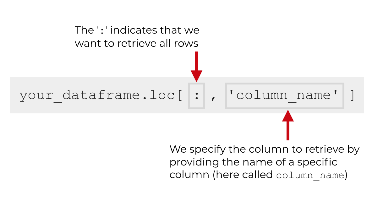
The next item inside of loc[] is the name of the column that we want to select.
This might still be a little abstract, so let’s take a look at a concrete example.
Example: how to select a single column using loc
In this example, we’re going to select the ‘population‘ column from the country_data_df DataFrame.
Here’s the code:
country_data_df.loc[:,'population']
And here is the output:
country
USA         322179605
China      1403500365
Japan       127748513
Germany      81914672
UK           65788574
India      1324171354
Name: population, dtype: int64
This is pretty straightforward.
We called the loc[] method by using dot notation after the name of the DataFrame, country_data_df.
Inside of the loc[] method, we have two arguments.
The first is the colon operator, which indicates that we want to retrieve all rows.
The second is the name of the column that we want to retrieve, population.
And what does it return? This code returns all of the row lables (which we set up as the country names earlier by using set_index('country'). It also returns the population that corresponds to each country.
Essentially, it returns the population column, along with the row labels, which looks like this:
![An image that show how the Pandas loc method returns a column of data when we use the code country_data_df.loc[:,'population'].](https://www.sharpsightlabs.com/wp-content/uploads/2019/02/pandas-loc-example-return-specific-column.png)
You can retrieve data in a similar way for the other columns … just use a different column name in place of ‘population.’ Change the code and try it out yourself!
Select a specific cell using loc
Next, let’s select the data in a single cell.
To select a single cell of data using loc is pretty simple, if you already know how to select rows and columns.
Essentially, we’re going to supply both a row label and a column label inside of loc[].
Let’s take a look:
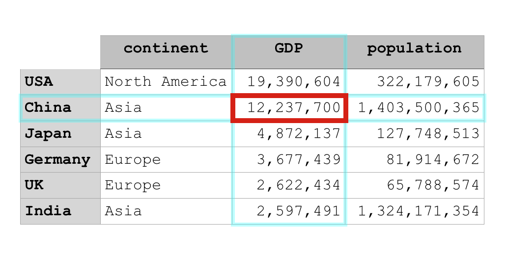
country_data_df.loc['China', 'GDP']
Which produces the following output:
12237700
This is pretty straightforward.
We called the loc[] method by using dot notation after the name of the DataFrame.
Inside of the method, we listed specified ‘China‘ as the row label and ‘GDP‘ as the column label.
This tells the loc method to return the data that meet both criteria. It tells loc to pull back the data that is in the ‘China‘ row and the ‘GDP‘ column. Visually, we can represent that like this:
Again … this is pretty simple once you understand the basic mechanics of loc.
Now though, let’s move on to something a little more complicated. Let’s talk about “slicing” DataFrames with the loc method.
Retrieve “slices” of data with loc
Instead of just retrieving single rows or single columns using loc, we can actually retrieve “slices” of data.
“Slices” of data are basically “ranges” of data.
The syntax for doing this is pretty easy to understand, if you’ve understood how to retrieve a single row.
How to retrieve a slice of rows using loc
Essentially, to retrieve a range of rows, we need to define a “start” row and a “stop” row.
Syntactically, you’ll call the loc[] method just like you normally would.
Then inside of the loc[] method, you’ll specify the label of the “start” row and the label of the stop row, separated by a colon.
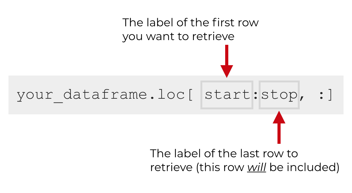
Keep in mind that the stop row will be included. The range of data that’s returned will be up to and including the stop row. This is different than how iloc[] works and how numeric indexes work generally in Python. Typically, the stop index is excluded, but that’s not the case with loc[].
Let me show you an example so you can see this in action.
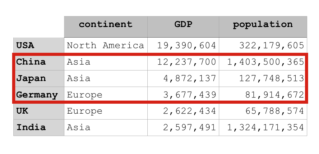
Example: retrieve a slice of rows using loc
Here, we’re going to retrieve a range of rows.
Specifically, we’ll retrieve the rows from ‘China‘ to ‘Germany‘.
Here’s the code:
country_data_df.loc['China':'Germany', :]
And here are the rows that it retrieves:
        continent       GDP  population
country
China        Asia  12237700  1403500365
Japan        Asia   4872137   127748513
Germany    Europe   3677439    81914672
As you can see, the code country_data_df.loc['China':'Germany', :] retrieved the rows from ‘China‘ up to and including ‘Germany‘.
Visually, we can represent the results of the code like this:
Next, let’s retrieve a slice of columns using loc.
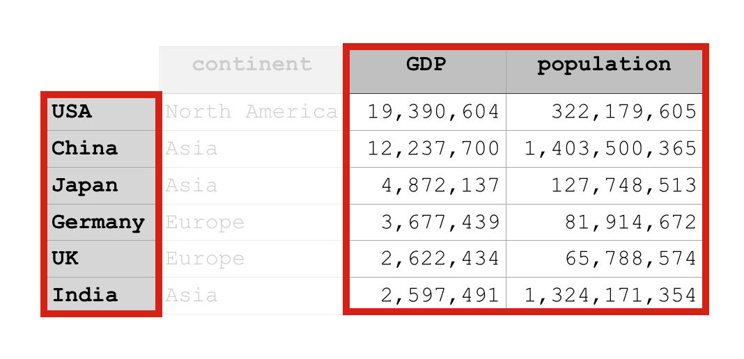
Example: retrieve a slice of columns using loc
Getting a subset of columns using the loc method is very similar to getting a subset of rows.
We’re going to call the loc[] method and then inside of the brackets, we’ll specify the row and column labels.
Because we want to retrieve all rows, we’ll use the colon (‘:‘) for the row label specifier.
After that, we’ll use the code 'GDP':'population' to specify that we want to select the columns from 'GDP' up to and including 'population'.
Here’s the exact code:
country_data_df.loc[:, 'GDP':'population']
Which produces the following result:
              GDP  population
country
USA      19390604   322179605
China    12237700  1403500365
Japan     4872137   127748513
Germany   3677439    81914672
UK        2622434    65788574
India     2597491  1324171354
Essentially, the code country_data_df.loc[:, 'GDP':'population'] retrieved all rows but only two columns, ‘GDP‘ and ‘population‘. It basically retrieved a “slice” of columns.
We can visually represent the output like this:
Finally, let’s put all of the pieces together and select a subset of cells using loc.
How to retrieve subsets of cells with loc
Selecting a subset of cells using the loc[] method is very similar to selecting slices.
Essentially, you’ll use code that returns a slice of rows and a slice of columns at the same time.
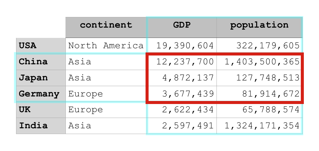
Let me show you an example.
Here is some code that will select the cells for GDP and population for the rows between China and Germany (including Germany).
country_data_df.loc['China':'Germany', 'GDP':'population']
Which produces the following output:
              GDP  population
country
China    12237700  1403500365
Japan     4872137   127748513
Germany   3677439    81914672
This is pretty simple to understand, if you already understand row slices and column slices. (If you don’t, go back and review those sections of this tutorial!)
We’ve called the loc method as normal.
Inside of loc[] we specified that we want to retrieve the range of rows starting from China up to and including the row for Germany.
After that, we then specified that we want to retrieve the columns for GDP up to and including the column for population.
We can visually represent the output like this:
Again, this is pretty easy to understand, as long as you understand the basics of the loc method.
Having said that, if you’re confused about anything in particular, leave your question in the comments at the bottom of this page.
Data manipulation is important, so master Pandas
Look.
You’ve probably heard it before …
Data manipulation is really important for data science.
If you want to be good at data science in Python, you really need to learn how to do data manipulation in Python.
That means that you need to learn and master Pandas. You should also learn more about NumPy.
I can’t stress this enough, if you want to learn data science in Python, make sure to study Pandas!
Sign up for our email list to learn more about Pandas
If you want to learn more about Pandas, and discover strategies to master Pandas, then sign up for our email list.
Every week here at Sharp Sight, we publish FREE data science tutorials.
We write about data science in Python … things like Pandas, matplotlib, NumPy and scikit learn.
(We also write about data science in R.)
If you want to learn more about data science, then sign up!
When you sign up for our email list, we send you our free data science tutorials every week.
You have nothing to loose … the tutorials are free, so sign up now.
This has to be the best explanation of this topic I’ve seen anywhere. I especially appreciate your small-step-by-small-step approach coupled with concrete examples.
Thanks so much. I look forward to learning more Python topics from your other tutorials.
Great to hear that this is useful.
Simple, concrete, and step-by-step is how we do things here.
And, there’s going to be a _lot_ more about Python in the future ….
NumPy, Pandas, data visualization, ML, deep learning …. a lot more to come.
I started a Data Science course last year and to be honest I have struggling to understand it. I have gone through dozens of sites on the internet but instead of helping me, I get confused the more.
I happened to stumble on this site by chance(of which I thank God for) while trying to understand how the random.rand and random.randn works.
It’s amazing how each topic is broken down to the tiniest bit. It’s simple, understandable and concise. I couldn’t have been happier.
Thank you Sharp Sight for this wonderful gift. Learning Data Science couldn’t have been better and more enjoyable for me if I had not found you.
You’re welcome. Good to hear that the explanations have helped.
Dear team, Thanks a lot for sharing such in a simple form.Please cover as much basic or topics as possible.. Again thanks a ton.
You’re welcome.
Excellent overview. Concise, clear and effective. A+
Great article
Thank you for the clear, basic explanation of loc. I’m just starting out with Pandas and this by far and away is the best explanation with clear examples. Great job!
There’s an ocean of blogs, then there is sharpsightlabs. Thank you, actually for creating this blog Josh :)
You have made Data Science so much more attainable. Reading through your blogs is a pleasure to understand any Data Science topic. People like me need a concise and clear explanation of what each letter, symbol, word in the syntax mean. And you do that in such a simplistic way, it is simply great.
Been following your blog for a while and also been a student of Datascience in R. Will keep coming back.
Thanks so much. Keep it going.
Thanks for the feedback, John.
Clear explanation is what we aim for here, and it’s good to hear that we’re hitting the mark.
Keep practicing and keep sharpening your skills
Such a nice and clear explanation in such detail!! A learner’s paradise.
Dear Joshua,
This page is crystal-clear, thanks a lot for it, it helped me a lot understanding the.loc[] features!
Just a question: when creating the example, you convert the dictionary into the df by: country_data_df = pd.DataFrame(country_data_dict, columns = [‘country’, ‘GDP’, ‘population’]).
Is the “columns = …” part necessary? – It seems to me that the DataFrame method already picks the dictionary keys as column index. Am I wrong?
You’re correct. And actually, your comment caused me to find a mistake in my code.
If you just use the
pd.DataFrame()function without thecolumns=parameter, the function will include all of the key/value pairs in the dictionary.You can alternatively use the
columns=to specify a subset of key/value pairs that you want to include. For example, the codecolumns = [‘country’, ‘GDP’, ‘population’]will only includecountry,GDP, andpopulation… but will excludecontinent.(Note: I changed the code to remove the columns parameter.)
You are missing to demonstrate following in code.
“Notice that in this step, we set the column labels by using the columns parameter inside of pd.DataFrame().”
You’re right. I had used the
columnsparameter in a previous version of this post, but I removed that parameter from the code a few months ago.After I changed the code, I didn’t update that line in the tutorial.
Now that you’ve pointed it out, I’ve removed that sentence.
loc is not a method, it is a property.
https://pandas.pydata.org/pandas-docs/stable/reference/api/pandas.DataFrame.loc.html
Don’t be pedantic.
Hello, I am grateful for this tutorial. I do have a question though. I was working with a dataset as a project and needed to call .loc on it after calculating the maximum average for each group in a row. I got the required output, but when I did a runner check with the expected output, I was informed that my output needs to look like a dictionary in python. Please how do I do about it. Thank you
I have no idea what you’re talking about here.
Try to post an example so I can see the issue.
Not at all sure what you mean by a “runner check”
What exactly did you do?