This tutorial will give you a quick introduction to the Pandas DataFrame.
At a high level, we’ll cover a few things:
- What Pandas is
- What Pandas DataFrames are
- How to create pandas DataFrames
- The basics of working with pandas DataFrames
Each of the above links will take you to the appropriate section, so if you’re looking for something specific, click on the link.
On the other hand, if you’re just getting started with Pandas and with data manipulation in Python, you should probably read the whole tutorial. Seriously. If you’re not in a hurry, just take a few minutes and read. Run some code. Stay a while.
Ok. Let’s get to it.
First, let’s just talk about Pandas.
What the hell is Pandas?
With all due respect to the people who create modules for programming languages, I think that the names of many packages are outright ridiculous.
Pandas? Why do pandas have anything to do with data?
I don’t know. I really don’t know.
In all seriousness, I think that the name Pandas confuses some beginners because it doesn’t have anything to do data. It’s not entirely clear what it’s about.
Let’s clear it up then.
Pandas is a data manipulation module for Python
Pandas is a data manipulation package for the Python programming language.
Pandas is actually one of a couple data manipulation packages in Python. The other core data manipulation package for Python is NumPy.
Pandas focuses on data frames
Although Pandas and NumPy both provide data manipulation tools, they focus on different things.
NumPy essentially focuses on numeric data that’s structured in an array. In fact, NumPy exclusively works with numeric data. Numeric data in Python. NumPy. Get it?
Importantly, NumPy arrays can be 1-dimensional, 2-dimensional, or multi-dimensional. So although they are limited in that they must contain numeric data, they are more flexible in that they can have an arbitrary number of dimensions. This can make them excellent for certain types of machine learning tasks (like deep learning).
Pandas, on the other hand, has a different focus. Pandas mostly focuses on a data structure called the “DataFrame,” which are strictly 2-dimensional (unlike the NumPy array), and contain heterogeneous columns (also unlike the NumPy array).
Now that we’re talking about the DataFrame, let’s discuss the two data structures of Pandas – the Series and the DataFrame – and how they are related.
Pandas has two data structures: Series and DataFrame
Pandas enables you to create two new types of Python objects: the Pandas Series and the Pandas DataFrame.
These two structures are related. In this tutorial, we’re going to focus on the DataFrame, but let’s quickly talk about the Series so you understand it.
A quick introduction to the Pandas Series
The Pandas Series object is essentially a 1-dimensional array that has an index.
In simpler terms, a Series is like a column of data. A column of data with an index.
Importantly, Series can contain data of any data type, as long as the all of the data in the Series have the same type. So a Series object can contain integers, strings, floats, etc … as long as all of the values have the same data type.
Again, you can think of a Series object as a column of data.
This brings us to the Pandas dataframe.
What is a Pandas dataframe?
So then … what is a dataframe?
In Python, a DataFrame is a 2-dimensional data structure that enables you to store and work with heterogeneous columns of data.
If that’s a little confusing, let me explain them a little differently:
Dataframes are like Excel spreadsheets in Python
Essentially, Pandas DataFrames are like Excel spreadsheets.
Here, I’m assuming that you’re familiar spreadsheets from Microsoft Excel.
Excel spreadsheets are fairly simple. They are 2-dimensional. And they have a row-and-column structure. All of the data are contained in columns that have the same data type.
Having said that, the different columns can have a different data type. So one column might have character data, and another column might have numeric data.
Pandas dataframes are 2-dimensional data structures
Pandas DataFrames are essentially the same as Excel spreadsheets in that they are 2-dimensional. They have a row-and-column structure. And the different columns can be of different data types.
Notably, Pandas DataFrames are essentially made up of one or more Pandas Series objects. Remember from a previous section that I mentioned how Pandas Series are like “columns” of data. Essentially, you can combine several of these column-like Series objects into a larger structure … a DataFrame.
Pandas dataframes have indexes for the rows and columns
When you’re working with dataframes, it’s very common to need to reference specific rows or columns. It’s also very common to reference ranges of rows and columns.
There are a couple of ways to do this, but one critical way to reference specific rows and columns is by index.
Every row and every column in a Pandas dataframe has an integer index.
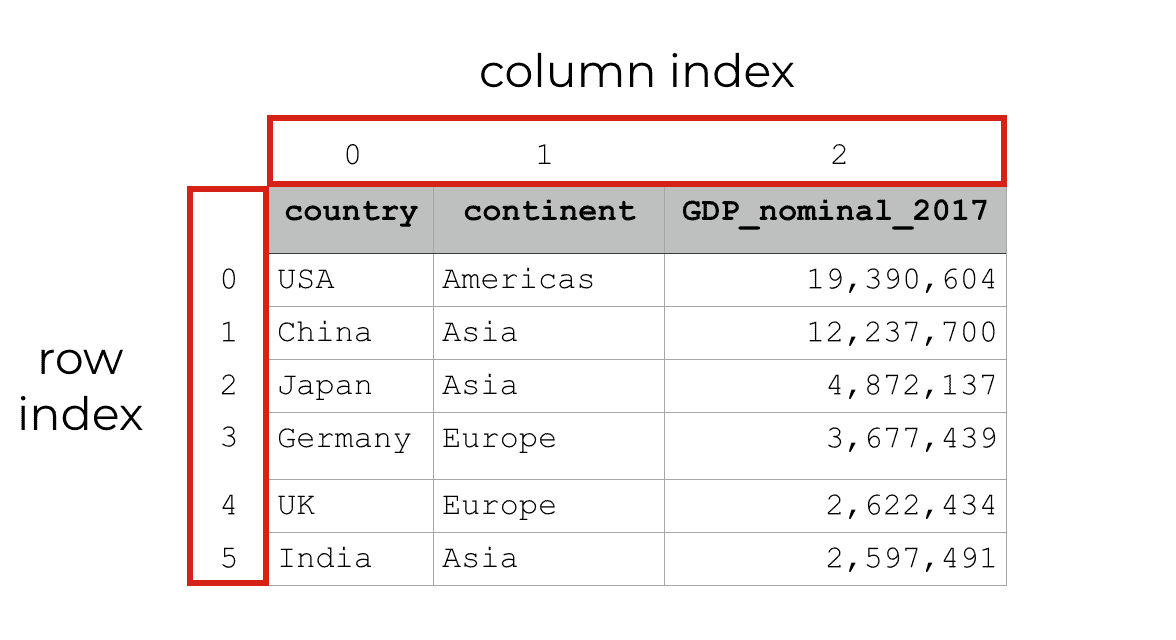
You can use these indexes to retrieve specific rows and specific columns by their number.
Similarly, you can use these index values to retrieve ranges of data. For example, you could retrieve rows 1 through 4.
Working with these numeric index values isn’t that complicated, but there’s a fair amount of material that you’ll need to know to do it properly.
Later in this tutorial, I’ll show you some simple examples of how to retrieve rows and columns by index.
For more detailed explanations, you should check out our tutorial on the Pandas iloc method and our tutorial on the Pandas loc method.
Pandas Dataframes give us flexibility for certain types of manipulations
You might be wondering, “why do we need DataFrames?”
As I noted earlier, DataFrames are more constrained than NumPy arrays in that they are strictly 2-dimensional. On the other hand, DataFrames can have different data types in different columns, whereas NumPy arrays need to have data that’s all of the same type.
So the structure of Pandas DataFrames makes them ideal for certain types of data tasks, and bad for others.
Specifically, Pandas DataFrames are good when you have heterogenious data.
Moreover, DataFrames are good when you need to perform certain types of tasks like:
- pivot tables
- groupings and aggregations
- visualizations
Again, DataFrames aren’t perfect for all data science tasks, but for some things they are ideal.
We’ll talk more about how to work with DataFrames later.
First though, let’s take a look at how to actually create DataFrames in Python.
How to create pandas dataframes
Ok. Here, we’re actually going to start working with some Python code.
We’ll start first by creating DataFrames with the Pandas module. Later in the tutorial, I’ll also show you some simple things that you can do to work with DataFrames.
But there’s one quick thing before we actually start working with the DataFrame code.
Quick reminder: import Pandas
Before running any of the example code in the following sections, you need to import Pandas into your working environment.
To do this, you can run the following code:
import pandas as pd
Here, we’ve imported Pandas with the alias pd. This is extremely common in Python code. When we import Pandas with an alias like this, we can type pd in our code instead of typing pandas. This simplifies things a little bit and makes your code a little easier to write.
Keep in mind that you could also import Pandas with the code import pandas, in which case you would refer to the Pandas module as pandas in your code.
Create DataFrame from a Python dictionary
First, let’s create a Pandas DataFrame from a python dictionary.
Create a Python dictionary
As our first step in creating a DataFrame from a dictionary, we’ll create a Python dictionary.
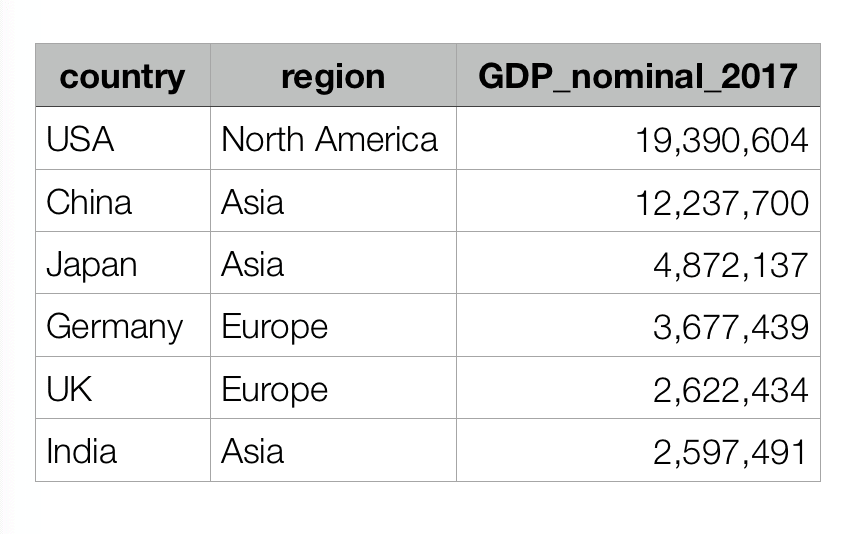
country_gdp_dict = {
    'country':['USA', 'China', 'Japan', 'Germany', 'UK', 'India']
    ,'GDP': [19390604, 12237700, 4872137, 3677439, 2622434, 2597491]
}
This dictionary has two different items. In both cases, the “key” is a string, and the “value’ is a list that contains some values associated with the key.
For example the word ‘country‘ is a key in our dictionary and the list of values (['USA', 'China', 'Japan', 'Germany', 'UK', 'India']) is the associated “value” of that key.
Essentially, when we turn this dictionary into a DataFrame, the key/value pairs will become the column name and the column data.
Before we do that though, let’s take a quick look at the data by using the print() function:
print(country_gdp_dict)
Which produces the following:
{'country': ['USA', 'China', 'Japan', 'Germany', 'UK', 'India']
, 'GDP': [19390604, 12237700, 4872137, 3677439, 2622434, 2597491]}
This dictionary contains a few rows of data about country-level nominal GDP, from Wikipedia: en.wikipedia.org/wiki/List_of_countries_by_GDP_(nominal).
From here, we can use the pandas.DataFrame function to create a DataFrame out of the Python dictionary.
Create a DataFrame from an existing dictionary
So now we have a dictionary that contains some data: country_gdp_dict.
Next, we’ll take this dictionary and use it to create a Pandas DataFrame object.
To do this, we’ll simply use the pandas.DataFrame function. Of course, because we’ve imported Pandas with the alias pd, we can call this function with the code pd.DataFrame().
country_gdp_df = pd.DataFrame(country_gdp_dict)
And we can examine the DataFrame by printing it out:
print(country_gdp_df)
Which produces the following output:
        GDP  country
0  19390604      USA
1  12237700    China
2   4872137    Japan
3   3677439  Germany
4   2622434       UK
5   2597491    India
Here, you can see the structure of the DataFrame.
The DataFrame has two columns: GDP and country.
The DataFrame has six rows of data, and each row has an associated index. Notice that the row indexes start at 0, so that the first row is row ‘0‘, the second row is row ‘1‘, etc. This is consistent with how Python handles indexes. The index values of essentially all Python objects start at 0. For example, the index values of Python lists and other sequences start at 0.
How to reorder the columns of the DataFrame
One other thing that I want to show you is how to re-order the columns of your DataFrame.
You might have noticed that the order of the columns in the final DataFrame was slightly different then the order we used when we created the dictionary that contained the data.
To fix this and give the columns a different order, you can use the columns parameter inside of the pd.DataFrame function.
country_gdp_df = pd.DataFrame(country_gdp_dict, columns = ['country','GDP'])
And if we print out the DataFrame, we will see the order of the columns:
print(country_gdp_df)
   country       GDP
0      USA  19390604
1    China  12237700
2    Japan   4872137
3  Germany   3677439
4       UK   2622434
5    India   2597491
Personally, I prefer this order. We’ll be looking at the data at a country level, so it helps to have the country variable in the first column position.
There are other ways to create pandas dataframes
Here, I’ve shown you one way to create a Python DataFrame with Pandas … we created a DataFrame from a dictionary of lists.
There are other ways to create Python DataFrames though. You can create DataFrames from dictionaries of Series objects, a dictionary of dictionaries, etc. Moreover, you can simply import data from csv files and other file types into a DataFrame.
Essentially, there are many ways to create Pandas DataFrames.
Having said that, I want to keep things simple here. Many of the other ways of creating DataFrames are less common or they require more explanation.
I’ll probably create separate tutorials to explain the other techniques.
Ok … now that I’ve shown you how to create a Python DataFrame, let’s look at some things that we can do with DataFrames.
Working with pandas dataframes
Working with DataFrames is a pretty broad subject. In fact, a lot of basic data science in Python involves working with DataFrames in one way or another.
With that in mind, this section isn’t going to tell you everything about working with data frames.
However, it will show you some of the basics. Here, I’ll show you how to get the column and row names from a pandas DataFrame. I’ll show you basic indexing, and also basic information retrieval.
Reminder: run this code
Just a quick reminder.
If you haven’t already done so, you need to import Pandas and create the DataFrame we’ll work with.
The following code is the same as the code above, so if you already ran it, you don’t need to. But if you haven’t run this already, go ahead.
Import pandas
Here’s the code to import Pandas.
import pandas as pd
Create data
And here’s the code to create the DataFrame that we’ll work with, country_gdp_df.
country_gdp_dict = {
    'country':['USA', 'China', 'Japan', 'Germany', 'UK', 'India']
    ,'GDP': [19390604, 12237700, 4872137, 3677439, 2622434, 2597491]
}

country_gdp_df = pd.DataFrame(country_gdp_dict, columns = ['country','GDP'])
Get the column names from a python DataFrame
Ok.
Here, we’re going to retrieve the column names from the DataFrame.
country_gdp_df.columns
Which produces the following output:
Index(['country', 'GDP'], dtype='object')
Essentially, when we retrieve the columns attribute from a Pandas DataFrame, it returns the columns. It returns the columns as a Pandas Index object.
I’m not going to explain Index objects in depth here, but you can treat these as sequences. This enables you to do things like retrieving a column name by it’s position. Let me show you how.
Get specific column name, by index
Here, we’ll retrieve the first column in the DataFrame. Remember, in Python, index values start at 0, so if we want to retrieve the first column name, we need to retrieve column 0.
So to retrieve the first column of country_gdp_df, we will request the 0th column, using bracket notation. It’s just like using a Python list.
country_gdp_df.columns[0]
Which produces the following column name:
'country'
Essentially, when we use the code country_gdp_df.columns[0], we are retrieving the first column name from the country_gdp_df DataFrame. Remember: the indexes for the column names start at 0, so the 0th column is the first column.
Get the row names from a python DataFrame
We can retrieve the row names from a DataFrame in a somewhat similar way.
One thing you need to know though: the row labels are called the “index” of the DataFrame. DataFrame indexes are a little technical and a little complicated for beginners, so in the interest of simplicity, I’m not going to write much about DataFrame indexes here.
What you really need to understand is that the index attribute returns the row names. And unless you’ve given the rows specific names (by specifying an index), the index attribute essentially returns the row number starting at 0.
Let me show you.
Here, we’re just going to retrieve the index parameter using Python dot notation after the name of the DataFrame:
country_gdp_df.index
Which produces the following output:
RangeIndex(start=0, stop=6, step=1)
Again, this returns a type of Index object, but if you take a look you can see that it is a range starting at 0 and stopping at 6, in steps of 1. Remember that in Python, index values are up to and not including the stop number. So essentially, this RangeIndex object includes the numbers from 0 to 5.
Inspecting dataframes
Before I wrap up this tutorial, I want to show you two do some basic data inspection with Pandas DataFrames.
Here, I’m going to show you two methods that you can use to inspect your data, head() and tail().
head()
The head method essentially prints out the first 5 rows of data.
To use it, you can specify the DataFrame you want to inspect, and then use the dot notation to call the head() method.
country_gdp_df.head()
Which produces the following output:
   country       GDP
0      USA  19390604
1    China  12237700
2    Japan   4872137
3  Germany   3677439
4       UK   2622434
Notice that this is the first 5 rows of data (rows 0 through 4).
tail()
You can also use the tail() method in a similar way to inspect the last 5 rows of data.
Here’s some code to use the tail method:
country_gdp_df.tail()
Which prints out the following rows:
   country       GDP
1    China  12237700
2    Japan   4872137
3  Germany   3677439
4       UK   2622434
5    India   2597491
Notice that these are the last 5 rows of data, rows 1 to 5. The first row – row 0, which is the row for the USA – has been omitted.
This doesn’t look like much here, but when you have a dataset with hundreds or thousands of rows (or more!) this method can be very useful.
How to select data from a Pandas dataframe
After reading about the basics of Pandas DataFrames here in this tutorial, one of the next things you need to learn is how to subset your data.
That being the case, I strongly recommend that you read the following tutorials next:
- How to use the
iloc[]method to subset a Pandas DataFrame - How to use the
loc[]method to subset a Pandas DataFrame
Those two tutorials will explain Pandas DataFrame subsetting. They can be a little complicated, so they have separate tutorials.
There’s a lot more to learn about Pandas DataFrames
In the interest of brevity, this is a fairly quick introduction to Pandas DataFrames.
Honestly, there’s a lot more that you can (and should) learn about DataFrames in Python.
As I already mentioned, you should read our other tutorials about subsetting Pandas DataFrames.
You should also learn some of the basics of data visualization … really, what good is a DataFrame if you don’t do anything with it?
You can learn more about data visualization in Python by reading about creating scatterplots, how to create a histogram in Python, and more.
Even beyond those other tutorials, there’s still a lot more to learn about data science in Python.
What else specifically do you want to learn about? Leave a comment in the comments section at the bottom of the page and tell me.
For more Python data science tutorials, sign up for our email list
Having said that, if you want to learn more about Pandas and more about data science in Python, sign up for our email list.
Here at Sharp Sight, we regularly post tutorials about data science topics. We have tutorials about data visualization and data manipulation. There are also regular tutorials about specific topics like Pandas, matplotlib, and more.
Additionally, we post articles about data science in R as well.
So if you’re serious about learning data science, sign up for our email list.
When you sign up, we’ll deliver our tutorials directly to your inbox, every week.
Good tutorial article, thanks! I would like to see some kind of guidance on how to learn/master matplotlib/seaborn libraries. I just started to learn how to do basic plot, but not very familiar to matplotlib’s structure and system.
BTW, pandas name is explained in the official document as –
“Panel is a somewhat less-used, but still important container for 3-dimensional data. The term panel data is derived from econometrics and is partially responsible for the name pandas: pan(el)-da(ta)-s….”
Panda is panel data
You are teaching the chained method to access elements in a DF, which i love btw. How do you retrieve 2 (or more columns) thought with this method? Lets say i query-filter some rows based on a logical condition and then i would like to see the output from 2(+) columns not just one
For one column i would have df.query(‘some logical condition).column_name.some_method
For 2+ columns? I’ve tried .column1.column2 (obviously doesnt work), neither .[‘column1′,’columns2’] (which – even if it worked – it would beat the purpose of chaining lines of code
Yeah, it doesn’t work your way. That’s why using “dot syntax” to access columns is bad.
The way to do it is with the .filter() method.
Specifically, use the filter method with a list of columns as the argument. You can find an example here:
https://www.sharpsightlabs.com/blog/pandas-filter/#example-2
Additionally, I recommend a better way to do method chains. There is a special syntax that enables you to chain together multiple Pandas methods on separate lines. This makes it easier to read, easier to write, and easier to debug.
Here’s an example:
(titanic
    .query('embark_town == "Southampton"')
    .filter(['sex', 'age', 'survived'])
    .sort_values(['age'], ascending = False)
)
This style of syntax is a lot like Dplyr pipes in R, and it’s very powerful, once you know how to use it properly.
You can read more about it here:
https://www.sharpsightlabs.com/blog/python-pandas/#pandas-chains
Simply written doc