Sklearn make_classification, Explained

With the rise of AI, machine learning has suddenly become very popular.

Machine learning has been around for decades, but machine learning systems are becoming increasingly important in a range of fields, from healthcare, to finance, to marketing.

Python, with a range of libraries for data science and ML, has arguably become the top language for machine learning. And the most popular machine learning library in Python is scikit-learn (often referred to as sklearn).

In this post, we’re going to take a close look at one particular function from scikit-learn: make_classification.

This tool helps us generate synthetic datasets for classification problems. This makes it very useful for practicing machine learning and evaluating machine learning algorithms.

We’ll look at what make_classification function does, how the syntax is structured, and I’ll also show you a simple example.

The blog post is divided into sections, and if you need anything specific, just click on one of the following links.

Table of Contents:

• Introduction
• Syntax
• Examples
• Frequently Asked Questions

That said, let’s dive into the sklearn make_classification function.

A Quick Introduction to Sklearn make_classification

The sklearn make_classification function allows Python users to create datasets that they can use for classification models.

It allows you to make data with binary labels and multiclass labels.

For example, here is a plot of a binary dataset that I made with make_classification:

(I’ll show you how to create this exact dataset later.)

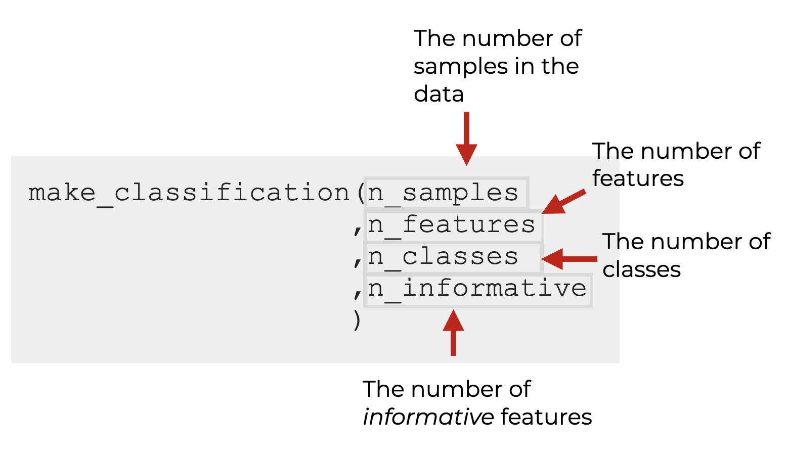
And importantly, it provides functionality that allows you to specify things like:

• the number of features
• the number of classes
• the number of informative features
• the number of examples
• … and many other details

Now that we’ve seen a brief overview of its capabilities, let’s delve deeper into the syntax of make_classification to understand how we can use it properly.

The Syntax of Sklearn make_classification

Here, I’m going to explain the syntax of the Scikit Learn make_classification function.

I’ll explain the high-level syntax, but also some of the details about the most important parameters.

A quick note

Everything I’m about to explain assumes that you have Scikit Learn installed on your machine, and that you’ve imported make_classification as follows:

from sklearn.datasets import make_classification

With that said, let’s look at the syntax.

make_classification syntax

The basic syntax, is very, very simple.

Assuming that you’ve imported the function as described above, you can call the function by typing make_classification().

There are a few important parameters as well that you can specify inside the parenthesis:

In some sense, the parameters are the most important part of the function, because they determine the exact structure and content of the output dataset.

That being the case, let’s quickly discuss the important parameters.

The Parameters of make classification

The Scikit Learn make classification function has quite a few parameters, but I believe that the most important are:

• n_samples
• n_features
• n_classes
• n_informative
• n_redundant
• class_sep
• n_clusters_per_class
• random_state

Let’s look at each of these, one at a time.

n_samples (required)

The n_samples parameter controls the number of samples in the output dataset.

Said differently, it controls the number of examples (or, the number of rows of data, if you’re thinking of a simple row-and-column dataset).

By default, this is set to 100.

n_features

The n_features parameter controls the number of features in the output dataset.

Remember, the features are like the inputs to a machine learning model. They are the columns that a machine learning algorithm learns from in order to make a prediction. Features are like the inputs to a model, and labels/targets are like the outputs of a model (to learn a bit more about features and labels, read our blog post on Supervised vs Unsupervised machine learning).

This will include the informative features, redundant features, and repeated features (if you use them when you create your dataset).

By default, this parameter is set to 20.

n_classes

The n_classes parameter controls the number of classes in the output dataset.

As mentioned above, the classes are the different possible categories for the target variable (remember that in supervised learning the dataset has a target/label variable that we’re trying to predict).

By default, this is set to n_classes = 2, so by default, make_classification will produce a binary dataset.

n_informative

The n_informative parameter controls the number of informative features in the output dataset.

So what does informative mean?

An informative feature is one that has a relationship with the target label. It carries information that enables us to learn how to predict the categorical values in the data.

So the rest of the features (the un-informative ones) may be noisy or otherwise irrelevant.

Introducing uninformative (or noisy) features into a dataset be useful, especially for experimental or educational purposes.

For example, uninformative features can:

• Make the dataset more realistic, since many real-world datasets have irrelevant features.
• Help with testing model robustness, since testing a model on data with irrelevant features can help gauge how it handles irrelevant inputs.
• Help with practicing feature selection, since we typically use feature selection to remove irrelevant features.
• Help test regularization, since regularization typically mitigates the effects of irrelevant or noisy featuers.

So it may sound a bit strange to have uninformative features, but if we’re making a dataset for machine learning practice or algorithm evaluation, it may actually be useful for the synthetic dataset to have uninformative features.

n_redundant

n_redundant enables you to specify how many redundant features there are.

It might seem odd, but redundant features can be useful if you’re practicing machine learning or testing a particular algorithm.

We can use redundant features to:

• Practice feature selection methods
• Evaluate model performance in the face of redundant features
• Evaluate the regularization ability of an algorithm

And more.

So like the “uninformative” features discussed earlier, redundant features can serve a useful purpose when we practice ML or try to evaluate algorithm performance.

class_sep

The class_sep parameter (short for “class separation”) controls the amount of separability between the generated classes.

There are some algorithm types where want (or need) the classes to be perfectly separable.

There are some algorithm types that allow the classes to overlap somewhat (so overlapping classes is good for testing such algorithms).

class_sep allows you to control the degree to which the classes overlap.

n_clusters_per_class

n_clusters_per_class allows you to specify how many clusters will be generated for every class.

By default, this is set to 2.

Why would you want to use this?

In some classification datasets, all of the data points for a particular class will form a tight “cluster”. They will be grouped together in feature space.

But other times, members of a single class might form multiple clusters of data … they might form separate groups.

Datasets where classes have multiple clusters are generally more complex, and a synthetic dataset with multiple clusters per class may be more “realistic.”

Essentially, the n_clusters_per_class parameter lets you emulate this complexity and real-worldness in the synthetic data created by make_classification.

random_state

The random_state parameter allows us to set a seed for the random number generator.

This ensures that any process or function that utilizes random numbers can be reproduced exactly every time we run it.

Essentially, this enables reproducibility when the code is run multiple times, whether by the same individual or different people.

If you want to learn more about seeds and random number generators, read our tutorial on Numpy Random Seed.

Other Parameters

There are several other features that I’m leaving out here for the sake of brevity, like weights, flip_y, hypercube, and several others.

However, many of these will be somewhat rarely used, so in the beginning, you may want to avoid using them unless absolutely necessary.

The Output of make_classification

The output of the Scikit Learn make_classification function is 2 Numpy arrays.

The first is a Numpy array with shape (n_samples, n_features). This is the so-called X array, which contains the feature data.

The second array is a Numpy array with shape (n_samples,). This is the so-called y array, which contains the labels. It’s essentially a vector of labels associated with every example in X. Importantly, the y array contains integers representing the classes, with the number of unique integers being determined by the n_classes parameter.

Examples of How to Use Make Classification

Now that I’ve shown you the syntax of make_classification, let’s look at a couple of examples.

Examples:

• Generate Data For Logistic Regression
• Create a 2D dataset with separated classes

Run this code first

Before you run the examples, make sure that you import the make_classification function with this code:

from sklearn.datasets import make_classification

import matplotlib.pyplot as plt
import seaborn as sns

Here, we’re also importing Seaborn and Matplotlib’s Pyplot, which we’ll use to visualize the data we generate.

Once you run it, you’ll be ready to get started.

EXAMPLE 1: Generate Data For Logistic Regression

Here, we’re going to generate some data that will be well suited for a Logistic Regression model.

We’re going to make a dataset with:

• 1000 examples (i.e., samples)
• 1 feature (an informative feature)
• 1 cluster per class
• mild class separation

And we’re going to initialize a random seed for the random number generator

X, y = make_classification(n_samples = 1000
                           ,n_features = 1
                           ,n_informative = 1
                           ,n_redundant = 0
                           ,n_clusters_per_class = 1
                           ,class_sep = 2
                           ,random_state = 2
                           )

And let’s visualize this data with a Seaborn scatterplot, so you can see it:

plt.style.use('fivethirtyeight')
sns.scatterplot(x = X.flatten(), y = y, hue = y)

OUT:

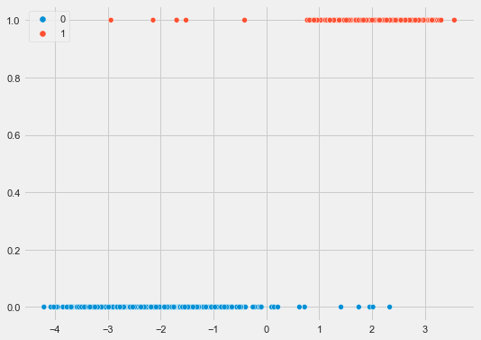
Here, we have a dataset with 1 feature and 2 classes.

We’ll be able to fit a logistic regression model to this, which I’ll show you how to do in a future blog post.

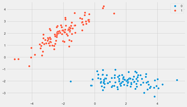
EXAMPLE 2: Create a 2D dataset with separated classes

In this example, I’m going to show you how to create a slightly more complicated dataset.

Here, we’ll create a dataset with:

• 200 examples (i.e., samples)
• 2 features (both of them informative features, 0 redundant)
• 1 cluster per class
• mild class separation

And again, we’ll use random_state to set a random seed for our random number generator (which will make the output of the code precisely reproducible).

Here’s the code to make the dataset:

X, y = make_classification(n_samples = 200
                           ,n_features = 2
                           ,n_informative = 2
                           ,n_redundant = 0
                           ,n_clusters_per_class = 1
                           ,flip_y = 0
                           ,class_sep = 2
                           ,random_state = 7
                           )

And let’s visualize the data:

plt.style.use('fivethirtyeight')

plt.figure(figsize = (10,6))
sns.scatterplot(x = X[:,0], y = X[:,1], hue = y, s = 50)

OUT:

As you can see, here, we have a dataset with 2 distinct classes.

There are several tools that we could use to classify this data, such as an SVM or a decision tree (although a decision tree would work better if we could rotate the data).

Frequently Asked Questions About make_classification

Do you have other questions about the Scikit Learn make classification function?

Is there something that I missed?

Are you still confused about something?

Leave your questions and comments in the comments section at the bottom of the page.

For more Python Machine Learning tutorials, sign up for our email list

In this blog post, I’ve shown you how to use Sklearn make_classification.

This is one simple tool for creating synthetic machine learning datasets.

But if you really want to master machine learning in Python, there’s a lot to learn.

That being said, if you want to learn more about ML and data science in Python, then sign up for our email list.

When you sign up, you’ll get free tutorials on:

• NumPy
• Pandas
• Base Python
• Scikit learn
• Machine learning
• Deep learning
• … and more.

So if you’re ready to master Python machine learning, then sign up now, and get our tutorials delivered direct to your inbox.