A Quick Introduction to Numpy Random Normal

This tutorial will cover the Numpy random normal function (AKA, np.random.normal).

If you’re doing any sort of statistics or data science in Python, you’ll often need to work with random numbers. And in particular, you’ll often need to work with normally distributed numbers.

The Numpy random normal function generates a sample of numbers drawn from the normal distribution, otherwise called the Gaussian distribution.

This tutorial will show you how the function works, and will show you how to use the function.

If you just need some help with something specific, you can skip ahead to the appropriate section with one of the following links:

Table of Contents:

• A quick introduction to Numpy Random Normal
• The syntax of numpy random normal
• Examples of how to use numpy random normal

But if you’re a little unfamiliar with Numpy, I suggest that you read the whole tutorial.

A Quick Overview of Numpy Random Normal

Let’s start with a high-level explanation of what Numpy Random Normal does.

A quick review of Numpy

Let’s briefly review what Numpy is.

Numpy is a module for the Python programming language that’s used for data science and scientific computing.

Specifically, Numpy performs data manipulation on numerical data. It enables you to collect numeric data into a data structure, called the Numpy array. It also enables you to perform various computations and manipulations on Numpy arrays.

Essentially, Numpy is a toolkit for creating and working with arrays of numbers in Python.

(For more details about Numpy array basics, check out our tutorial about the NumPy array.)

Numpy random normal generates normally distributed numbers

So Numpy is a package for working with numerical data in Python.

Where does np.random.normal fit in?

As I mentioned previously, Numpy has a variety of tools for working with numerical data. In most cases, Numpy’s tools enable you to do one of two things: create numerical data (structured as a Numpy array), or perform some calculation on a Numpy array.

The Numpy random normal function enables you to create a Numpy array that contains normally distributed data.

A Quick Review of Normally Distributed Data

Hopefully you’re familiar with normally distributed data, but just as a refresher, here’s what it looks like when we plot it in a histogram:

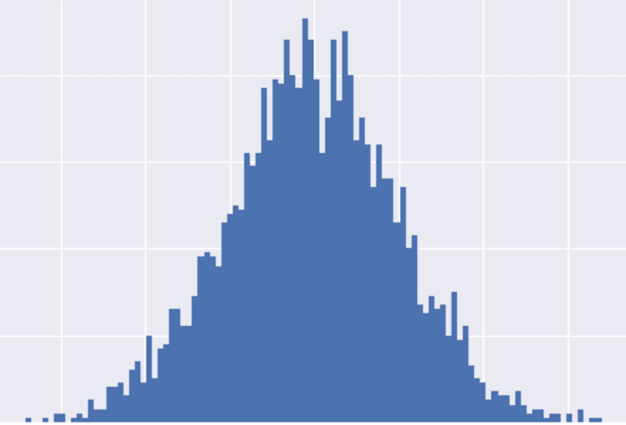
Normally distributed data is shaped sort of like a bell, so it’s often called the “bell curve.”

2 Important Parameters for the Normal Distribution

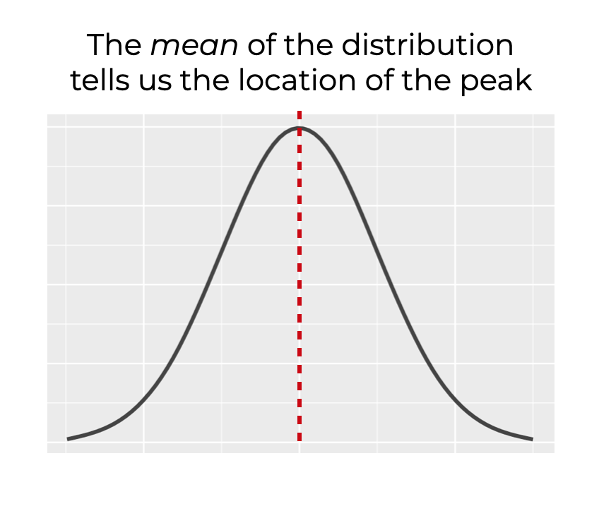
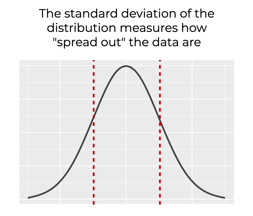
Importantly, there are 2 primary parameters that influence the shape of the distribution:

• mean
• standard deviation

The mean tells us where the peak of the distribution is.

The standard deviation measures how “spread out” the data are (although, there are other metrics that measure the spread of the data, like variance).

These metrics are both important, because they relate directly to two syntactical parameters of Numpy random normal.

So to tie this back to np.random.normal, the Numpy random normal function allows us to create normally distributed data, while specifying important parameters like the mean and standard deviation.

With that in mind, let’s look at the a look at the syntax.

The Syntax of Numpy Random Normal

The syntax of the Numpy random normal function is fairly straightforward.

Note that in the following syntax explanation and throughout the rest of this blog post, we will assume that you’ve imported Numpy with the following code: import numpy as np. That code will enable you to refer to Numpy as np.

np.random.normal syntax

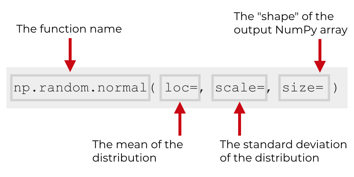
Here’s the basic syntax:

Let me explain.

Typically, we will call the function with the name np.random.normal(). As I mentioned earlier, this assumes that we’ve imported Numpy with the code import numpy as np.

Inside of the function, you’ll notice 3 parameters: loc, scale, size.

These allow you to control the mean, the standard deviation, and the size/shape of the normal distribution, respectively.

Let’s talk about each of those parameters.

The parameters of the np.random.normal function

The np.random.normal function has three primary parameters that control the output: loc, scale, and size.

I’ll explain each of those parameters separately.

loc

The loc parameter controls the mean of the output data.

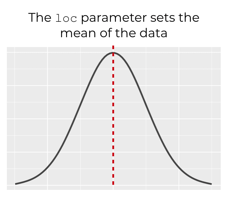
This parameter defaults to 0, so if you don’t use this parameter to specify the mean of the distribution, the mean will be at 0.

(I’ll show you an example of this in example 4.)

scale

The scale parameter controls the standard deviation of the normal distribution.

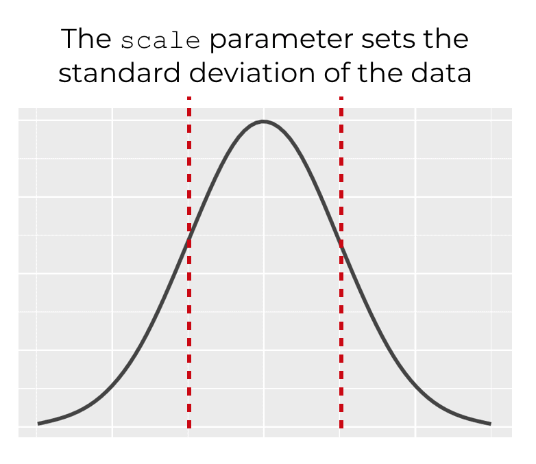
By default, the scale parameter is set to 1.

(I’ll show you an example of this in example 5.)

size

The size parameter controls the size and shape of the output.

Remember that the output will be a Numpy array. Numpy arrays can be 1-dimensional, 2-dimensional, or multi-dimensional (i.e., 2 or more).

This might be confusing if you’re not really familiar with Numpy arrays. To learn more about Numpy array structure, I recommend that you read our tutorial on Numpy arrays.

Having said that, here’s a quick explanation.

The argument that you provide to the size parameter will dictate the size and shape of the output array.

If you provide a single integer, x, np.random.normal will provide x random normal values in a 1-dimensional Numpy array.

You can also specify a more complex output.

For example, if you specify size = (2, 3), np.random.normal will produce a Numpy array with 2 rows and 3 columns. It will be filled with numbers drawn from a random normal distribution.

Keep in mind that you can create output arrays with more than 2 dimensions, but in the interest of simplicity, I will leave that to another tutorial.

(I’ll show you an example of this in parameter in example 3.)

Examples: how to use the Numpy random normal function

Now that I’ve shown you the syntax the Numpy random normal function, let’s take a look at some examples of how it works.

Examples:

• Draw a single number from the normal distribution
• Draw 5 numbers from the normal distribution
• Create a 2-dimensional Numpy array of normally distributed values
• Generate normally distributed values with a specific mean
• Generate normally distributed values with a specific standard deviation
• Combined example that uses the loc, scale, and size parameters

Run this code before you run the examples

Before you work with any of the following examples, make sure that you run the following code:

import numpy as np

I briefly explained this code at the beginning of the tutorial, but it’s important for the following examples, so I’ll explain it again.

The code import numpy as np imports the Numpy module into your working environment and enables you to call the functions from Numpy. If you don’t use the import statement to import Numpy, Numpy’a functions will be unavailable.

Moreover, by importing Numpy as np, we’re giving the Numpy module a “nickname” of sorts. So we’ll be able to refer to Numpy as np when we call the Numpy functions.

You probably understand this if you’ve worked with Python modules before, but if you’re really a beginner, it might be a little confusing. So, I wanted to quickly explain it.

A quick note about Numpy Random Seed

In several of these examples, you’ll see me use np.random.seed to set the seed for Numpy’s random number generator.

I’m doing this so that the output of the code is “repeatable.” If you use the same seed that I do in these examples, you should get the exact same output (but if you use a different seed value, you will get different output).

We often use np.random.seed for repeatability, particularly in the context of tutorials.

If you want to read more about Numpy random seed, you can check out our tutorial about the np.random.seed function.

Ok, now let’s work with some examples.

Example 1: Draw a single number from the normal distribution

First, let’s take a look at a very simple example.

Here, we’re going to use np.random.normal to generate a single observation from the normal distribution.

np.random.normal(1)

This code will generate a single number drawn from the normal distribution with a mean of 0 and a standard deviation of 1.

Essentially, this code works the same as np.random.normal(size = 1, loc = 0, scale = 1).

Remember: if we don’t specify values for the loc and scale parameters, they will default to loc = 0 and scale = 1.

Example 2: Draw 5 numbers from the normal distribution

Now, let’s draw 5 numbers from the normal distribution.

This code will look almost exactly the same as the code in the previous example.

np.random.normal(5)

Here, the value 5 is being passed to the size parameter. It indicates that we want to produce a Numpy array with 5 values, drawn from the normal distribution.

Also note that because we have not explicitly specified values for loc and scale, they will default to loc = 0 and scale = 1.

Example 3: Create a 2-dimensional Numpy array of normally distributed values

Now, we’ll create a 2-dimensional array of normally distributed values.

To do this, we need to provide a tuple of values to the size parameter.

np.random.seed(42)
np.random.normal(size = (2, 3))

Which produces the output:

array([[ 1.62434536, -0.61175641, -0.52817175],
       [-1.07296862,  0.86540763, -2.3015387 ]])

So we’ve used the size parameter with the size = (2, 3). This has generated a 2-dimensional Numpy array with 6 values.

This output array has 2 rows and 3 columns. Here, the “2” in the input tuple specified the number of rows, and the “3” specified the number of columns.

In this example, we used the size parameter to create a 2-dimensional array. But be aware that you can use the size parameter to create arrays with higher dimensional shapes.

Example 4: Generate normally distributed values with a specific mean

Now, let’s generate normally distributed values with a specific mean. To do this, we’ll use the loc parameter.

Recall from earlier in the tutorial that the loc parameter controls the mean of the normal distribution from which the function draws the numbers.

Here, we’re going to set the mean of the data to 50 with the syntax loc = 50.

np.random.seed(42)
np.random.normal(size = 1000, loc = 50)

The full array of values is too large to show here, but here are the first several values of the output:

array([ 50.49671415,  49.8617357 ,  50.64768854,  51.52302986,
        49.76584663,  49.76586304,  51.57921282,  50.76743473,
        49.53052561,  50.54256004,  49.53658231,  49.53427025 
...

You can see at a glance that these values are roughly centered around 50. If you were to calculate the average using the Numpy mean function, you would see that the mean of the observations is 50.

Example 5: Generate normally distributed values with a specific standard deviation

Next, we’ll generate an array of values with a specific standard deviation.

As noted earlier in the blog post, we can modify the standard deviation by using the scale parameter.

In this example, we’ll generate 1000 values with a standard deviation of 100.

np.random.seed(42)
np.random.normal(size = 1000, scale = 100)

And here the first few values of the output:

array([  4.96714153e+01,  -1.38264301e+01,   6.47688538e+01,
         1.52302986e+02,  -2.34153375e+01,  -2.34136957e+01,
         1.57921282e+02,   7.67434729e+01,  -4.69474386e+01
...

Notice that we set size = 1000, so the code will generate 1000 values. I’ve only shown the first few values for the sake of brevity.

It’s a little difficult to see how the data are distributed here, but we can use the std() method to calculate the standard deviation:

np.random.seed(42)
np.random.normal(size = 1000, scale = 100).std()

Which produces the following:

99.695552529463015

If we round this up, it’s 100.

Notice that in this example, we have not used the loc parameter. Remember that by default, the loc parameter is set to loc = 0, so by default, this data is centered around 0. We could modify the loc parameter here as well, but for the sake of simplicity, I’ve left it at the default.

Example 6: Combined example that uses the loc, scale, and size parameters in np.random.normal

Let’s do one more example to put all of the pieces together.

Here, we’ll create an array of values with a mean of 50 and a standard deviation of 100.

np.random.seed(42)
np.random.normal(size = 1000, loc = 50, scale = 100)

I won’t show the output of this operation …. I’ll leave it for you to run it yourself.

Let’s quickly discuss the code. If you’ve read the previous examples in this tutorial, you should understand this.

We’re defining the mean of the data with the loc parameter. The mean of the data is set to 50 with loc = 50.

We’re defining the standard deviation of the data with the scale parameter. We’ve done that with the code scale = 100.

The code size = 1000 indicates that we’re creating a Numpy array with 1000 values.

Frequently asked questions about np.random.normal

Now that you’ve learned about np.random.normal and seen some examples, let’s review some frequently asked questions about the function.

Frequently asked questions:

• What’s the difference between np.random.normal and np.random.randn?

Question 1: What’s the difference between np.random.normal and np.random.randn

You might have seen a different function for creating normally distributed data in Python, called np.random.randn.

The np.random.randn function is related to np.random.normal, but there are some differences.

Just like np.random.normal, the np.random.randn function produces numbers that are drawn from a normal distribution.

The major difference is that np.random.randn is like a special case of np.random.normal. np.random.randn operates like np.random.normal with loc = 0 and scale = 1.

So this code:

np.random.seed(1)
np.random.normal(loc = 0, scale = 1, size = (3,3))

Operates effectively the same as this code:

np.random.seed(1)
np.random.randn(3, 3)

Said differently, np.random.randn is a special function that generates data from the “standard normal” distribution.

If you have other questions, leave your question in the comments section

Is there something that I’ve missed here?

Are you still confused about something specific about Numpy random normal?

If so, leave your question or comment in the comments section at the bottom of the page.

If you want to learn data science in Python, learn Numpy

So that’s it. You can use the Numpy random normal function to create normally distributed data in Python.

But if you really want to master data science and analytics in Python, you need to learn more about Numpy.

The np.random.normal function is just one piece of a much larger toolkit for data manipulation in Python.

Having said that, if you want to be learn more, you can check out our other Numpy tutorials on things like:

• How to create a Numpy array
• How to reshape a Numpy array
• How to create an array with all zeros
• How to use Numpy arrange
• How to use Numpy linespace
• How to append one Numpy array to another

And more…

For more Python data science tutorials, sign up for our email list

More broadly though, if you want to learn data science in Python, you should sign up for our email list.

Here at Sharp Sight, we regularly post tutorials about a variety of data science topics. In particular, we regularly publish tutorials about Numpy.

If you sign up for our email list, we will send our Python data science tutorials directly to your inbox.

You’ll get free tutorials on:

• Numpy
• Matplotlib
• Pandas
• Base Python
• Scikit learn
• Machine learning
• Deep learning
• … and more.

Want to learn data science in Python? Sign up now.