The confusion matrix is an important and commonly used tool in machine learning. This is particularly true of classification problems, where we build systems that predict categorical values.
Because they’re used so frequently for classification problems, you need to know them, and you need to know them well.
So in this blog post, I’m going to explain confusion matrices.
I’ll explain what they are, how we use them, how they’re structured, and a lot more.
For the sake of simplicity, I’ve divided the tutorial up into sections. If you want to learn something specific, you can click on one of the following links, and it will take you to the appropriate section.
Table of Contents:
- A Quick Review of Classification
- Explanation of How Classifiers Can Make Different Types of Correct and Incorrect Predictions
- A Quick Review of True Positive, True Negative, False Positive and False Negative
- The Confusion Matrix: a Tool To Evaluate Classifiers
- How to Interpret the Quadrants of a Confusion Matrix
- Final Thoughts
Having said that, it’s probably best to read everything, since you’ll need to know a bit of background information about how classifiers work in order to really understand confusion matrices and why they’re important.
With that said, let’s jump in.
A Quick Review of Classification
Before we talk about confusion matrices, let’s quickly review classification.
I’m sure that you know (since you’re a smart and hard-studying data science student), that a classifier predicts categories.
This is in contrast to a regressor (for example, linear regression), which predicts numeric values.
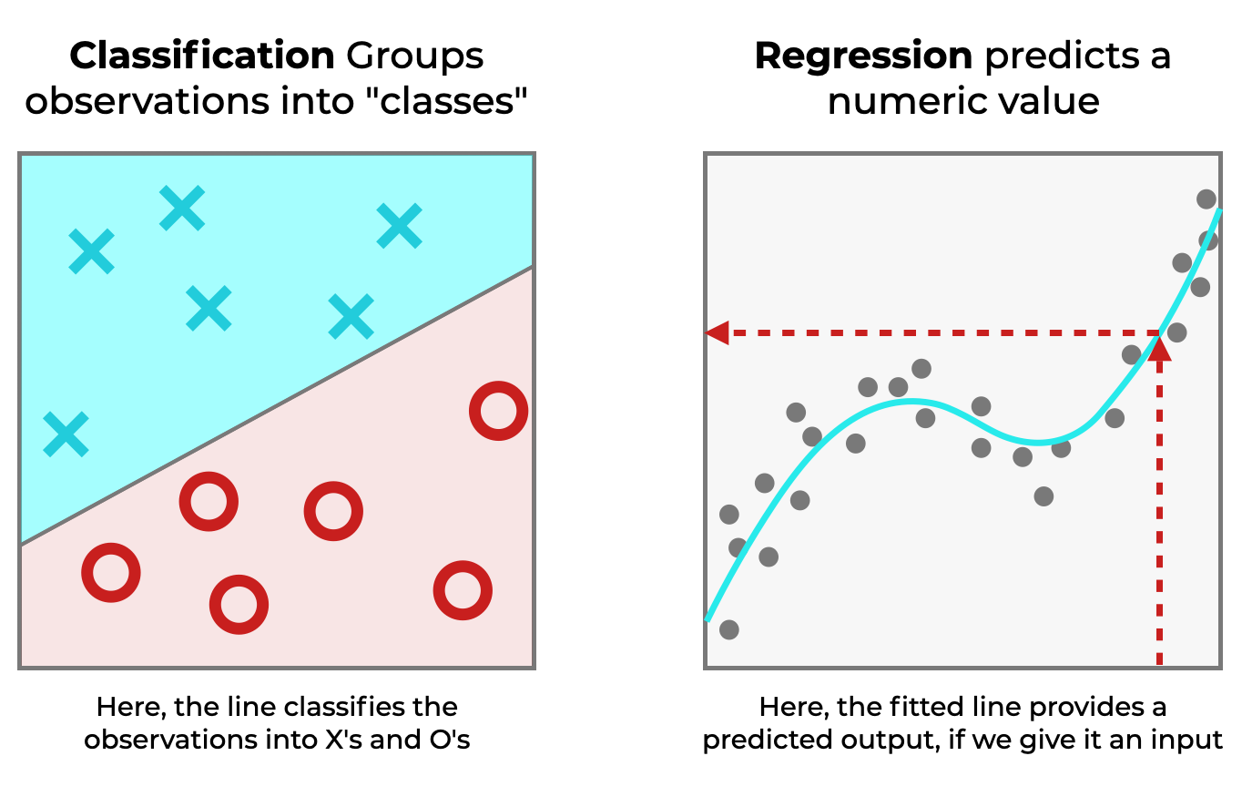
Regression and classification are two types of machine learning tasks.
But for our purposes, classification is the important one here, because we use confusion matrices for classification systems.
A Quick Example of a Classification System
To help you understand classification, let’s think up a simple example.
Imagine you built a machine learning system that classifies images. It’s a simple binary classifier. It inputs images and classifies every image as “cat” or “not cat“.
We’ll call it, The Cat Classifier.
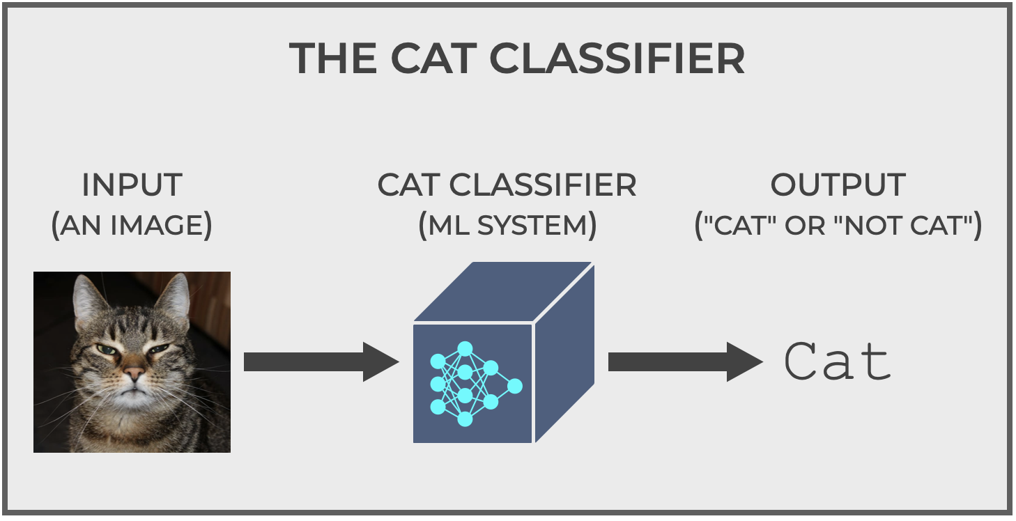
All this system does is accept images as input and output a prediction: cat or not cat.
And importantly, those predictions might be correct or incorrect.
Different types of correct predictions and incorrect predictions
Understanding correct and incorrect predictions of classifiers is vital for understanding the confusion matrix.
You’ll see why soon, but first, let’s go back to our hypothetical Cat Classifier. We’ll use it to look at the types of correct predictions and incorrect predictions. This in turn will build the conceptual understanding you’ll need to understand confusion matrices.
Ok. Back to our hypothetical Cat Classifier.
Remember that the Cat Classifier makes predictions of cat or not cat.
You feed it an image, and it predicts cat or not cat.
As we already discussed, it’s possible to make a correct prediction (e.g., the input is actually an image of a cat, and the classification system correctly predicts cat).
It’s also possible to make incorrect predictions (e.g., the actual image is something like a dog, but the classification system incorrectly predicts cat).
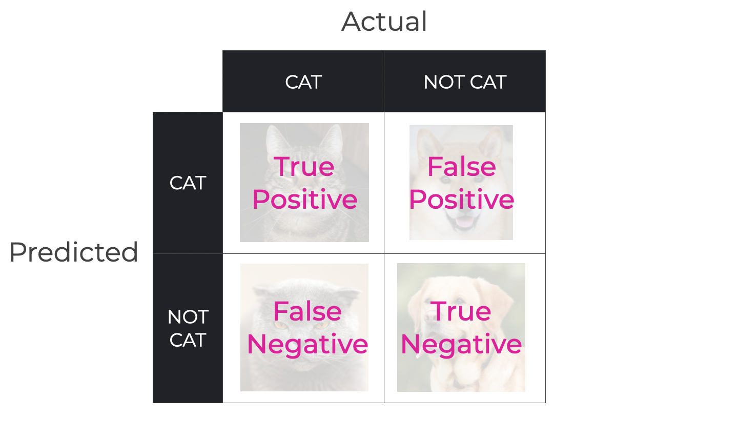
In fact, if we have a binary classification system like our Cat Classifier, there are actually four types of classification outcomes.
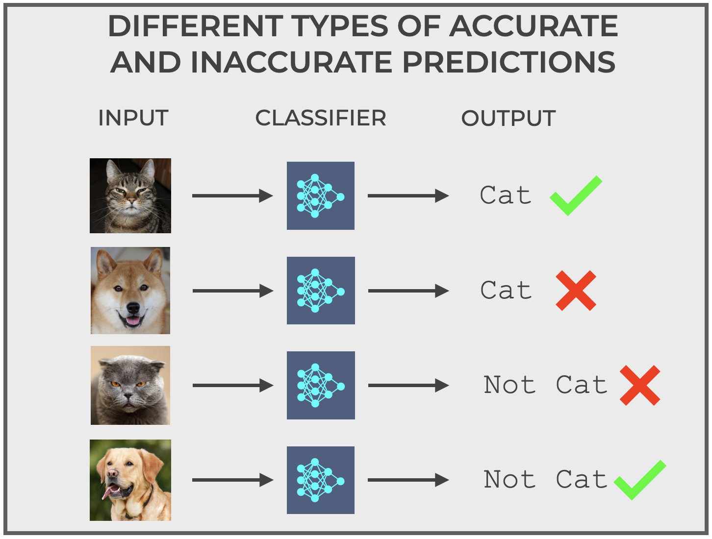
As you can see above, there is:
- Correctly predicting
catwhen the actual input iscat - Correctly predicting
not catwhen the actual input isnot cat - Incorrectly predicting
catwhen the actual input isnot cat - Incorrectly predicting
not catwhen the actual input iscat
For example, the second image is a Shiba Inu … a type of dog with pointy ears and short fur.
It’s a dog, so the actual value for the purposes of our model is not cat, but let’s hypothetically assume that our classification makes a mistake, and predicts cat. It’s a mistake.
Alternatively, the third image is actually a cat, but a bit of a strange cat. It’s an image of a Scottish Fold cat. Scottish Fold is a breed that has small, flopped over ears.
It’s an image of a cat, so the actual value is cat, but let’s assume that the classifier makes a mistake and predicts not cat. Again, this is a particular type of mistake.
So we have different types of correct and incorrect predictions.
True Positives, True Negatives, False Positives and False Negatives
These different types of correct and incorrect predictions I mentioned above all have names.
To talk about this, let’s generalize our binary prediction system.
Instead of talking about cat vs not cat, we can label binary outcomes as positive and negative (i.e. cat becomes positive and not cat becomes negative).
By generalizing binary classification labels to positive and negative, we can describe the different types of correct and incorrect predictions in the following ways:
- True Positive (TP): A positive case that is correctly predicted as positive
- True Negative (TN): A negative case that is correctly predicted as negative
- False Positive (FP): A negative case that is incorrectly predicted as positive (Type I Error).
- False Negative (FN): A positive case that is incorrectly predicted as negative (Type II Error).
These will be essential when I finally show you a confusion matrix in a later section.
We’re almost there.
A Grid of Correct and Incorrect Prediction Types
Next, let’s take the different types of predictions and organize them into a grid.
(I swear, we’re getting close to talking about confusion matrices.)
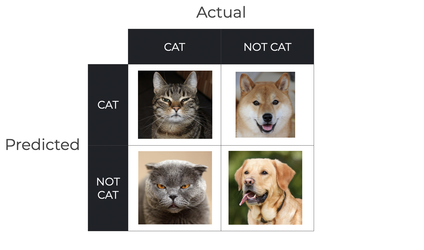
We can organize our grid according to the actual value (which has 2 possible values, cat and not cat) and the predicted value (which also has 2 possible values, cat and not cat).
When we organize the observations this way, according to actual value and predicted value, we get a 2×2 grid.
We’re getting close … this is almost a confusion matrix.
Just bear with me a little while longer.
A Grid of True Positives, True Negatives, False Positives and False Negatives
Finally, remember what I wrote a few sections ago about the different types of correct and incorrect predictions:
- True Positive (TP): A positive case that is correctly predicted as positive
- True Negative (TN): A negative case that is correctly predicted as negative
- False Positive (FP): A negative case that is incorrectly predicted as positive (Type I Error).
- False Negative (FN): A positive case that is incorrectly predicted as negative (Type II Error).
Every location in our 2×2 grid corresponds to one of those prediction types.
And finally … we’re at a point where I can explain the confusion matrix.
The Confusion Matrix: A tool for evaluating binary classification
So this brings us to the confusion matrix.
A confusion matrix is a visual tool that we can use to evaluate the performance of a binary classifier.
Specifically, it counts up the true positives, true negatives, false positives, and false negatives.
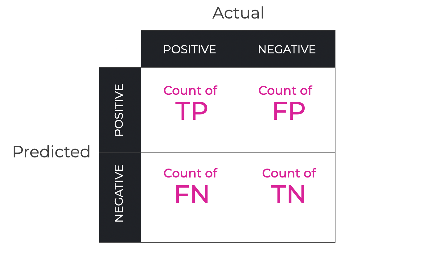
This allows us to evaluate the extent to which a classification system is making accurate predictions, and if not, what kinds of incorrect predictions it’s making.
How to Use the Quadrants of a Confusion Matrix
The different quadrants of a confusion matrix offer different insights:
- TP & TN: These two quadrants represent correct predictions, representing the model’s accuracy (in fact, these quadrants are related to the metric that we call accuracy, which is an important classification metric).
- FP: This quadrant measures instances when the model incorrectly identified a negative case as positive. These cases are what we would commonly call “false alarms.”
- FN: This quadrant measures instances where the classifier failed to identify a positive case, incorrectly classifying it as negative. This is sometimes called a “miss,” in the sense that the model is missing something that’s actually there.
Importantly, False Positives and False Negatives can have different costs and different consequences, depending on the exact task.
For example, in a medical setting, a false negative in a cancer detection task could have dire consequences.
Alternatively, in a military setting, a false positive might be very costly for a missile defense system. Imagine if a missile defense system indicated that an attack was incoming, but it was just a flock of birds. This sort of false alarm, if it triggered an unnecessary military response, could have very expensive, even disastrous consequences economically or geopolitically.
So it’s important to note that different systems optimize for different quadrants.
Sometimes you’re optimizing for accuracy (getting the most TP or TN).
Other times you might optimize for avoiding false positives or false negatives.
It depends on the task.
But, in any of these situations, the confusion matrix is a powerful tool for understanding and improving the performance of your classification model.
Related Concepts and Additional Considerations
I have to be honest.
I could have continued writing, and then continued writing some more.
There’s so much that I’m leaving out here, because there are many other things about confusion matrices that we could discuss.
In the interest of brevity, I’m going to cut this blog post short, but there are a few related topics that I’ll briefly mention.
Metrics Related to the Confusion Matrix
There are several classification performance metrics that are related to confusion matrices, including:
- Accuracy: Overall correctness of the model ((TP+TN) / Total).
- Precision: Accuracy of positive predictions (TP / (TP+FP)).
- Recall (AKA, Sensitivity): The model’s ability to detect all positive instances (TP / (TP+FN)).
- F1 Score: Harmonic mean of Precision and Recall, ideal for imbalanced datasets.
- Specificity: Ability to correctly identify negative instances (TN / (TN+FP)).
- False Positive Rate: Proportion of negative instances wrongly classified as positive (FP / (FP+TN)).
- False Discovery Rate: Proportion of positive predictions that were false (FP / (FP+TP)).
Most of these are important for evaluating and improving classification models, especially under particular circumstances.
Each of these metrics provides a different lens to help us evaluate a classifier’s performance.
Having said that I’ll write more about each of these in the future.
Multiclass Confusion Matrices
In this blog post, I’ve focused almost exclusively on binary classification, and my discussion of confusion matrices has therefore centered on how we use them for binary classifiers.
But, you should know that we can extend confusion matrices to multiclass classification problems.
Briefly, if you had n classes instead of 2 classes, then your confusion matrix would be an nxn grid instead of a 2×2 grid.
The principles of how we construct and interpret a multiclass confusion matrix are essentially the same as the binary case, but the interpretation becomes more difficult and more nuanced. For example, we often need to break the matrix down with a one-vs-all approach.
Again, this is somewhat more complex, so in the interest of brevity, I’ll write about it more later.
How to Use a Confusion Matrix to Improve Classifier Performance
Using the information of a confusion matrix to improve a model is somewhat complicated, and it depends on the exact task.
But briefly, we can use a confusion matrix to identify the weak spots of a classifier, and improve it.
For example, we can use a confusion matrix when we:
- Adjust Decision Thresholds: Altering the probability threshold can help optimize for precision or recall.
- Balance Training Data: Ensuring equal representation can mitigate biases.
Limitations of Confusion Matrices
Finally, let’s quickly talk about the limitations of confusion matrix.
Although confusion matrices are useful tools for evaluating performance of classifiers, they do have limitations.
This is especially true when we use them for models built on imbalanced datasets. In such a case, model could appear to be very accurate if one class dominates the dataset. The high accuracy could be misleading due to the dominance of one class.
Additionally, as noted above, when you build a classifier, you need to understand the real-world costs and consequences of false positives and false negatives. A confusion matrix might be able to help you identify problems with FNs and FPs, but only knowledge of the problem space can tell you how important those problems are, and how you might need to use that information to better align the model’s performance with the goal of the system.
Final Thoughts
Confusion matrices are a powerful and also commonly used tool to evaluate classification systems.
As you learn and master machine learning, you will need to understand how to use the confusion matrix to evaluate and optimize your models.
That said, this blog should have helped you understand what they are and how they are structured.
And additionally, hopefully I’ve given you a little insight into how we can use them.
But as noted previously, if you’re serious about mastering machine learning, then there’s a lot more to learn about confusion matrices, so I’ll be writing more about them in the future.
Leave Your Questions and Comments Below
Do you have other questions about the confusion matrix?
Is there something that’s confusing?
Do you wish that explained something else?
I want to hear from you.
Leave your questions and comments in the comments section at the bottom of the page.
Sign up for our email list
If you want to learn more about machine learning (including more about confusion matrices), then sign up for our email list.
Several times per month, we publish free long-form tutorials about a variety of data science topics, including:
- Scikit Learn
- Pandas
- Numpy
- Machine Learning
- Deep Learning
- … and more
If you sign up for our email list, then we’ll deliver those free tutorials to you, direct to your inbox.
Very educative, clearly explained and short. Thanks
You’re welcome.