F1 Score, Explained

If you want to master modern machine learning and AI, one of the major sub-areas that you need to master is classification.

Classification is one of the most important types of task in machine learning and AI.

But mastering classification, in part, means mastering how to evaluate classification systems.

Which in turn, means understanding the wide range of classification evaluation metrics.

That brings us to F1 score.

F1 score is one of the most important classification evaluation metrics and you need to know it well.

So in this post, I’m going to tell you all of the essentials that you need to know about F1 score.

I’ll explain what F1 is, the pros and cons of F1, how to improve it, and more.

If you need something specific, just click on any of these links and the link will take you to the appropriate point in the post.

Table of Contents:

• A Quick Review of Classification
• F1 Score Basics
• Pros and Cons of F1 Score
• How to Improve F1 Score
• Alternatives to F1 Score

Having said that, F1 score is sometimes a little challenging to understand, so it would probably be helpful if you read the whole post.

Ok. Let’s get to it.

A Quick Review of Classification

First, before we directly discuss F1 score, we should really review what classification is and how it works.

Everything you need to know about F1 hinges on a solid understanding of classification and different types of classification predictions (both correct and incorrect predictions).

So here, we’ll quickly review classification and then move on to F1 score (and obviously, if you’re 100% positive that you know all of this cold, then you can just skip ahead).

Machine Learning Overview

Quickly, let’s discuss what machine learning is, since that frames our discussion of classification.

Machine learning is the discipline of building computer systems that improve their performance when we expose them to data.

So machine learning systems are different from traditional computer programs.

Whereas in a traditional computer system, a human programmer explicitly programs all of the computer’s steps, in a machine learning system, we set up an algorithm that’s capable of “learning” as we expose it to data examples.

ML systems can learn to do a variety of tasks, but one of the most common tasks is classification.

What is Classification

Classification systems (also known as “classifiers”) learn to categorize (AKA, classify) input examples by predicting a categorical label.

In classification, the potential labels come from a pre-defined list. For example:

• spam or not spam
• cat or not cat
• fraud or not fraud
• positive or negative

In classification, we already know the possible labels, and we just want the system to predict the correct label every time we give it an example.

To better understand this, let’s look at an example.

A quick example of classification

The example that I like to use to explain how classification works is something that I like to call “The Cat Detector.”

The Cat Detector is simple.

It detects cats.

More specifically, you feed the Cat Detector images and it outputs only one of two possible outputs:

• positive (which indicates that it thinks the image is a cat), or
• negative (which indicates that it things the image is not a cat).

It’s a very simple binary classifier.

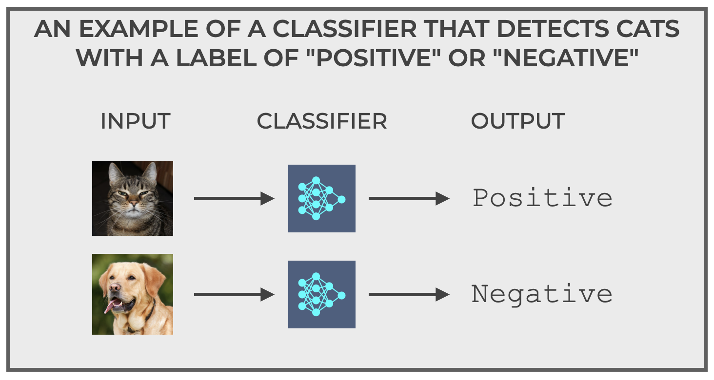
Input an image, output a prediction of cat or not a cat (i.e., positive or negative)

Having said that, in spite of the seeming simplicity, it is a little more complicated than it appears.

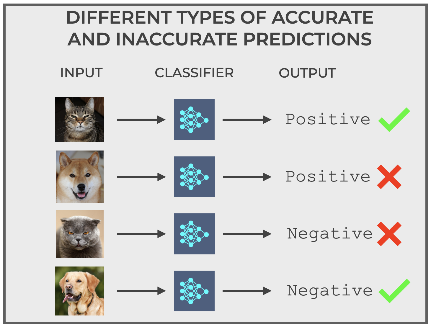
Classification Mistakes

The main thing that makes classification systems more complicated is that essentially all classifiers make mistakes (unless the task is trivially easy).

Said another way, classification predictions are sometimes incorrect.

To show this, let’s go back to our Cat Detector system.

In a perfect world, you’d feed the Cat Detector a picture of a cat, and it would always output positive.

And you’d feed the Cat Detector a picture of a non-cat (like a dog), and it would always output negative.

But that’s the idealized, perfect behavior.

And that perfect behavior never happens when we’re working on difficult, real world problems.

In the real world, with hard problems, our classifier will make mistakes.

For example, you might show the Cat Classifier an image of a cat, but it outputs negative, indicating that it predicts not-a-cat.

Or, you might show the Cat Classifier an image of a non-cat (such as a dog), and it outputs positive, indicating that it (incorrectly) predicts that the image is a cat.

So in the real world, our binary classifier actually has 4 different prediction types … 2 “correct” prediction types, and 2 “incorrect” prediction types, as shown here:

At this point, you might be asking yourself “So what? Classifiers make mistakes. How does this relate to F1 Score?”

Good question.

We’re getting there …

We just need to talk a little more specifically about these correct and incorrect prediction types.

Because they’re at the core of classifier evaluation, and therefore, at the core of F1.

Just bear with me a little bit more, and we’ll get to F1.

Correct and Incorrect Prediction Types

The correct and incorrect prediction types that we just saw with the Cat Detector can be generalized for all binary classifiers.

Remember that for the Cat Detector, there are 4 types of predictions:

• Correctly predict positive when the input is actually a cat
• Correctly predict negative when the input is not a cat
• Incorrectly predict positive when the input is not a cat
• Incorrectly predict negative when the input is actually a cat

But if we generalize the possible input classes for any binary classifier as positive and negative, and also generalize the possible output predictions for any binary classifier as positive and negative, then predictions of any binary classifier will fall into one of these 4 groups, according to the actual class of the input and the predicted class of the output:

• True Positive: Predict positive when the actual input is positive
• True Negative: Predict negative when the actual input is negative
• False Positive: Predict positive when the actual input is negative
• False Negative: Predict negative when the actual input is positive

And note that each of these four prediction types has a name, True Positive, True Negative, False Positive, and False Negative.

Why does this matter?

Because almost all classification metrics and classification evaluation tools are built on True Positives, True Negatives, False Positives, and False Negatives.

Accuracy, precision, recall, confusion matrices …

They all depend on the numbers of these prediction types.

And for the purposes of this blog post, so does F1 score.

F1 Score Basics

Ok.

We’re finally ready to talk about F1 score.

F1 score is a classification metric that enables us to evaluate the performance of a classifier.

This measure, which is widely used to evaluate of classification models, balances between precision and recall, two other classification metrics.

Quick Review of Precision and Recall

To understand F1, you need to understand precision and recall.

Precision measures the proportion of positive predictions (i.e., model output predictions) that were actually positive.

(1)  

You can think of precision as the accuracy of the positive predictions.

On the other hand, recall (AKA, sensitivity) is the proportion of positive examples that were correctly classified as positive.

(2)  

(Do you see why we needed to understand True Positives, False Positives, and False Negatives?)

The Problems of Precision or Recall

Although precision and recall can both be informative for evaluating classifiers, they both offer a one-sided view of a model’s performance. This frequently leads to misleading conclusions if considered in isolation.

Precision focuses on the correctness of the positive predictions made by the classifier. High precision indicates that when the model predicts a positive value, it’s likely correct. However, a model can achieve high precision simply by being overly conservative in making positive predictions. Said differently, if a classifier makes fewer positive predictions, only when it’s extremely confident that the positive prediction is correct, it can achieve high precision. But doing so might miss many actual positive cases. This can be particularly problematic in situations where failing to detect positive examples has very high cost, like in diagnosing a deadly disease.

Recall, on the other hand, assesses the model’s ability to properly detect all of the actual positive examples. A high recall means that the model is good at capturing positive cases. However, high recall fails to consider the cost of false positives. In some situations, like spam detection, excessive false positives (i.e., labeling a normal email that you want to get as “spam”) can be a big inconvenience.

Again: optimizing a classifier strictly for high precision or high recall can cause problems.

F1 Score: A Balance Between Precision and Recall

Enter F1 Score.

F1 score balances between precision and recall.

It does this because it’s computed as the harmonic mean of precision and recall, where the harmonic mean is:

(3)  

Therefore, F1 score can be computed as:

(4)  

Which simplifies to:

(5)  

And by plugging in the quantities for True Positive, False Positive, and False Negative (and with a bit of math), we can compute F1 score as follows:

(6)  

(Again: do you see why it’s important to understand True Positives, False Positives, and False Negatives?)

F1 provides a metric that balances between minimizing FN and FP

Ultimately, F1 score harmonizes between both precision and recall. It provides a single metric that measures the model’s overall efficiency in correctly identifying positives, while also minimizing both false positives and negatives.

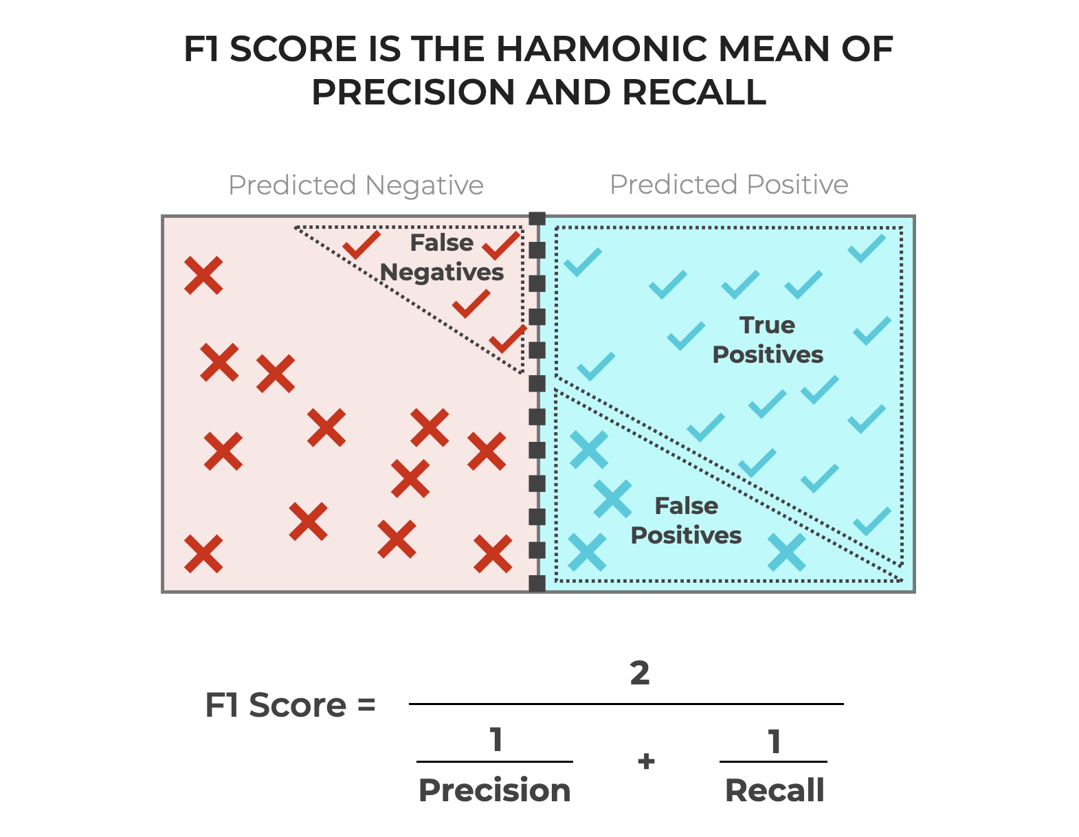
By using the harmonic mean, F1 score ensures that a model performs well in both precision and recall to perform well on this metric.

This balance is critical in many practical applications where both False Positives and False Negatives have substantial costs.

Therefore, F1 score offers a more comprehensive metric to evaluate a classifier’s performance, which makes it a preferred metric for many machine learning and AI applications.

An Example of F1 Score

To illustrate how we F1 is calculated, let’s look at a simple example.

Let’s assume that we’re using the Cat Detector model that I described above.

We’ll assume that the model has already been trained, and we’re evaluating how the model works on a new dataset.

To do this, we’ll use 100 photos as input examples. Among these 100 examples are 50 pictures of dogs (non-cats) and 50 pictures of cats.

We’ll feed the pictures into the Cat Detector and let the system predict whether or not the image is a cat or non-cat.

After doing this, the Cat Detector produces these output predictions (shown here as a confusion matrix):

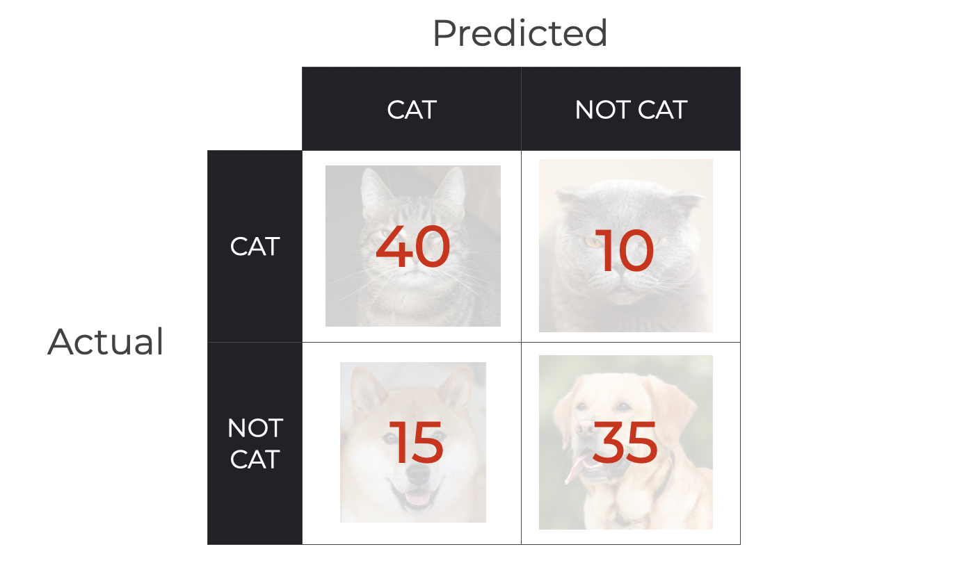
So, we have the following predictions:

• 40 True Positives (pictures of cats predicted as cat)
• 15 False Positives (pictures of non-cats predicted as cats)
• 35 True Negatives (pictures of non-cats predicted as not cat)
• 10 False Negatives (pictures of cats predicted as not cat)

Using these numbers, and in particular, using the number of True Positives, True Negatives, and False Negatives, we can calculate F1.

Calculating F1 Score with TP, TN, FP, and FN

So, let’s calculate the F1 Score of our classifier using the quantities shown above, and using equation 6 seen earlier.

(7)  

Plugging in the numbers, we get:

(8)  

Which gives us:

(9)  

So the F1 Score of our system is .76.

Wrapping Up: Why F1 Score is a Useful Metric

F1 score is often superior to precision recall because it takes a balanced approach in evaluating classifier performance.

While precision measure the accuracy of the positive predictions, precision doesn’t directly account for the number of actual positive examples that the model fails to predict.

Recall, on the other hand, assess the ability to correctly identify all of the positive examples, but it overlooks the proportion of positive predictions that were actually correct, which can increase the number of False Positives.

F1 score, being the harmonic mean of both precision and recall, mitigates these limitations by accounting for both precision and recall at the same time. And by doing this, F1 score provides a more wholistic assessment of the performance of a classifier.

Further Reading

If you want to learn more about classification evaluation, you should read our posts about:

• Precision
• Recall
• ROC Curves
• Confusion Matrices

Additionally, I’m going to write more about F1 score in the future, to cover topics like how to improve F1 score, when to use F1 score (and when not to), and more.

Leave Your Questions and Comments Below

Do you have other questions about F1 score?

Are you still confused about something, or want to learn something else about F1 that I didn’t cover?

I want to hear from you.

Leave your questions and comments in the comments section at the bottom of the page.

Sign up for our email list

If you want to learn more about machine learning and AI, then sign up for our email list.

Every week, we publish free long-form tutorials about a variety of machine learning, AI, and data science topics, including:

• Scikit Learn
• Numpy
• Pandas
• Machine Learning
• Deep Learning
• … and more

If you sign up for our email list, then we’ll deliver those free tutorials to you, direct to your inbox.