How to Make a Python Perceptron from Scratch

The Perceptron stands as one of the most basic building blocks for creating neural networks, including more advanced structures like deep networks and their variants.

Originally developed in the late 1950s, Perceptrons were designed to mimic the function of biological neurons.

I recently wrote a blog post explaining some of the history of Perceptrons as well as how Perceptrons work conceptually.

But in this blog post, I’m going to show you how to build a Python Perceptron, step by step and from scratch.

Here’s a quick table of contents so you can navigate to the right section if you just need something quick.

Table of Contents:

Prerequisites and Required Knowledge
Full Perceptron Code
Step-by-Step Code Explanation
Concluding Remarks

Prerequisites and Required Knowledge

To get the most out of this blog post, you’ll need to know a few things:

Perceptron Conceptual Basics
Base Python
Numpy
Python Class Construction
Data Visualization

Now to be clear, you can still review this blog post if you’re missing some of that knowledge.

You can even read the blog post if you’re missing all of the knowledge.

But it will be much easier to understand if you know a little about them.

Perceptron Conceptual Basics

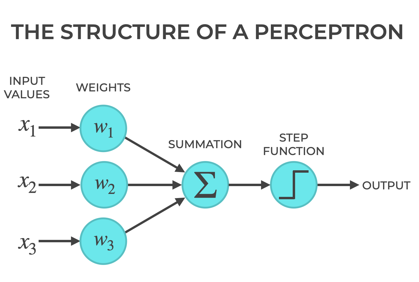
First, you’ll need to know a little about how Perceptrons work and how they’re structured.

At a high level, a Perceptron inputs numbers, weights those inputs, sums the weighted inputs, and then applies a step function to determine if the perceptron is on or off.

Of course, what I just wrote is extremely high level, and it would probably help to get further explanation about the meaning of terms like weights, bias, activation function, etc.

You can find all of that information in my previous blog post, Perceptrons Explained.

Base Python

You’ll also need to know several elements of Base Python.

In particular, you’ll need to know the basics of variable assignment, tuple assignment (which we’ll use briefly), and for loops.

For loops will be particularly necessary, because we’re going to need to use for loops when we write the code to “train” our Perceptron over multiple iterations.

Along with this, it will be useful to know a bit about functions that we use in for loops, like enumerate().

Numpy

You’ll also need to know a bit about Numpy.

In particular, you’ll need to know about:

It will also be good to know about Numpy array shapes.

You’ll need all of this because our Perceptron will be largely built on Numpy arrays. We’ll use Numpy arrays as inputs, we’ll use Numpy arrays as the weights and biases, and we’ll use Numpy functions to operate on our Perceptron during training and prediction.

I’ll explain more of those details as we work through the code.

Python Class Construction

In addition to Base Python and Numpy, you should probably know a bit about how we construct classes in Python.

In our code, we’re essentially going to create a new Perceptron class from scratch, along with methods to initialize a perceptron, train the perceptron on input data, and make predictions.

Again, you probably need to know a little bit about:

how classes are structured
how to write an initialization method
how to write custom instance methods (to operate on the class)

Data Visualization

Finally, it would be helpful to know a little bit about Python data visualization.

Specifically, we’re going to use Seaborn and some helper functions from Matplotlib to visualize our data.

We’re going to create some scatterplots and some decision boundaries (i.e., lines).

I’ll reiterate that you can probably get along fine if you’re missing some of the above prerequisite skills, but it will be much easier to understand everything if you already know them.

Python Perceptron Code

Ok. Let’s get into the code for our Python Perceptron.

I’m going to explain all of these parts, but here’s the full code for the Perceptron class:

import numpy as np

class Perceptron():
    def __init__(self, learning_rate = .01, n_iterations = 1000):
        self.learning_rate = learning_rate
        self.n_iterations = n_iterations
        self.bias = None
        self.weights = None
        
    
    def activation_function(self, net_input):
        # STEP ACTIVATION
        return np.where(net_input > 0, 1, 0)
    
    
    def fit(self, features, targets):
        n_examples, n_features = features.shape
        
        # change these to use different initialization scheme
        self.weights = np.random.uniform(size = n_features, low = -0.5, high = 0.5)
        self.bias = np.random.uniform(low = -0.5, high = 0.5)
        
        for _ in range(self.n_iterations):
            for example_index, example_features in enumerate(features):
                net_input = np.dot(example_features, self.weights) + self.bias
                y_predicted = self.activation_function(net_input)
                self._update_weights(example_features, targets[example_index], y_predicted)
        
        
    def _update_weights(self, example_features, y_actual, y_predicted):
        error = y_actual - y_predicted
        weight_correction = self.learning_rate * error
        self.weights = self.weights + weight_correction * example_features
        self.bias = self.bias + weight_correction
        
    def predict(self, features):
        net_input = np.dot(features, self.weights) + self.bias
        y_predicted = self.activation_function(net_input)
        return y_predicted

Let’s break this down piece by piece.

Step by Step Code Explanation

Here, I’m going to break down every part of our Python Perceptron code, step by step.

There’s a lot going on here, and there’s several different parts, but I’m going to keep it as clear an organized as possible.

As always, if you have questions about my explanation, leave your questions in the comments at the bottom of the page.

Import Packages

First, we need to import Numpy, since we’ll be using several Numpy tools as we create our perceptron.

import numpy as np

Class Initialization

The first several lines are just the initialization of the class.

class Perceptron():
    def __init__(self, learning_rate = .01, n_iterations = 1000):
        self.learning_rate = learning_rate
        self.n_iterations = n_iterations
        self.bias = None
        self.weights = None

We’re literally using the class keyword to define the Perceptron class.

Then immediately after that, we’re defining an initialization method, __init__().

In Python, __init__() is a special method name. It defines what happens when we initialize a new instance of the method. So what you see here is what happens when we call the Perceptron() code to create a new instance of the Perceptron class.

Look closely.

We’re using the ‘self‘ parameter several times. You’ll see that a lot.

self allows us to initialize specific properties of our class when we first create an instance of it.

(If you don’t know what all this is, you probably need to learn more about Python class construction … these are Python foundations.)

So what are we doing here?

Our Python Perceptron has a few attributes that exist at initialization:

learning_rate
n_iterations
bias
weights

As you look at these attributes, remember the structure of a perceptron.

A perceptron has inputs, and every input is associated with a weight. We also often have a bias term, which you can think of as a weight, but one that’s not associated with an input.

So we’ve designed our Perceptron to have a weight attribute and a bias attribute. These are both set to None at initialization because we haven’t assigned any values yet. We’re creating the attribute now, and we’ll pass data to these attributes later.

We also have a learning rate and the number of iterations.

These will be used for training.

Most neural network structures (from Perceptrons to large deep neural network architectures) learn over multiple iterations. And they also typically use a learning rate, which is the size of the step that the learning algorithm takes when it updates the weights.

Choosing good values for learning rate and the number of iterations is important for building a model that is accurate as well as computationally efficient. Having said that, learning rate and learning iterations can be a little difficult to understand at first, so I’ll explain more about them in separate blog posts.

Suffice it to say, learning rate and the number of iterations are important for training our neurons, and here at initialization, we’re giving these attributes some default values.

Later on, you’ll see us use these attributes in other parts of our code.

Define Activation Function

In this section of the code we’re defining the activation function.

In this case, we’re hard-coding a step function.

    def activation_function(self, net_input):
        # STEP ACTIVATION
        return np.where(net_input > 0, 1, 0)

As I explained in my previous blog post about Perceptrons, a perceptron takes in the input values, weights the inputs, sums up the weighted inputs, and then passes that summed input to the activation function.

The activation function evaluate the input and conditionally turns on if the net input (the sum of all weighted inputs, plus the bias term) reaches a certain threshold.

Notice that one of the input values to the method is called net_input. This is literally the “net input” to the activation function … the input values times the weights, plus the bias term. We calculate this net input elsewhere in the Perceptron class (in the fit() method), so you’ll see it again.

Once we pass the net_input into the method, we have the code for our activation function.

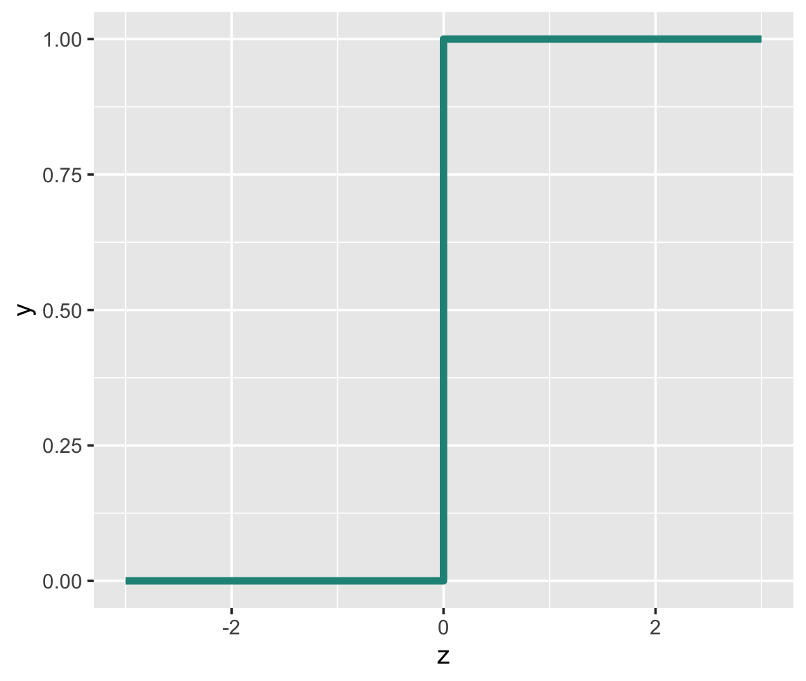
In this case, our activation function is a step function.

So:

if the net input is greater than 0, the activation function outputs a 1
if the net input is less than or equal to 0, the activation outputs a 0.

This is what our activation function looks like:

Syntactically, to implement this step function, we’re using the Numpy where function.

Numpy where operates conditionally. It has a condition, and it outputs one value if the condition is true, and a different value if the condition is false.

So, net_input is passed into the method, and we operate on it with Numpy where.

Here, our condition is net_input > 0. So if net_input is greater than 0, Numpy where outputs a 1, else it outputs a 0.

And ultimately, the output of Numpy where is the output of our activation function.

A Quick Note About Activation Functions

The step function is a common and traditional activation function for artificial neurons and neural networks.

We’re using it here because it’s simple and commonly used for Perceptrons in particular.

Having said that, there are many, many different activation functions, including:

ReLU
Logistic Sigmoid
Softplus
Elu (Exponential Linear Unit)
Selu (Scaled Exponential Linear Unit)
Leaky Relu
Random leaky Relu

… and others.

Each of these are structured differently, and have different uses.

Some are good for deep neural networks.

Some are traditionally used for deep networks, but sometimes cause problems.

Some of these activation functions fix common problems with network training.

And so on.

Different activation functions are used for different purposes, and they have different strengths and weaknesses.

So activation functions are important, and you eventually need to learn more about them.

But for now, we’re going to stick to the step function, because it’s easy to use, and common for Perceptrons.

Fit Method

Ok.

This part is gonna suck.

It’s the hardest part to understand, because it’s here that we actually implement the learning part of our little Perceptron machine learning system.

Before we get to it, let me quickly remind you what learning is. To paraphrase something found in the book Deep Learning, learning is a process by which a system improves performance on a task as it is exposed to data.

So here, we’re going to define how our Perceptron can improve its performance as a classifier as we expose it to training examples.

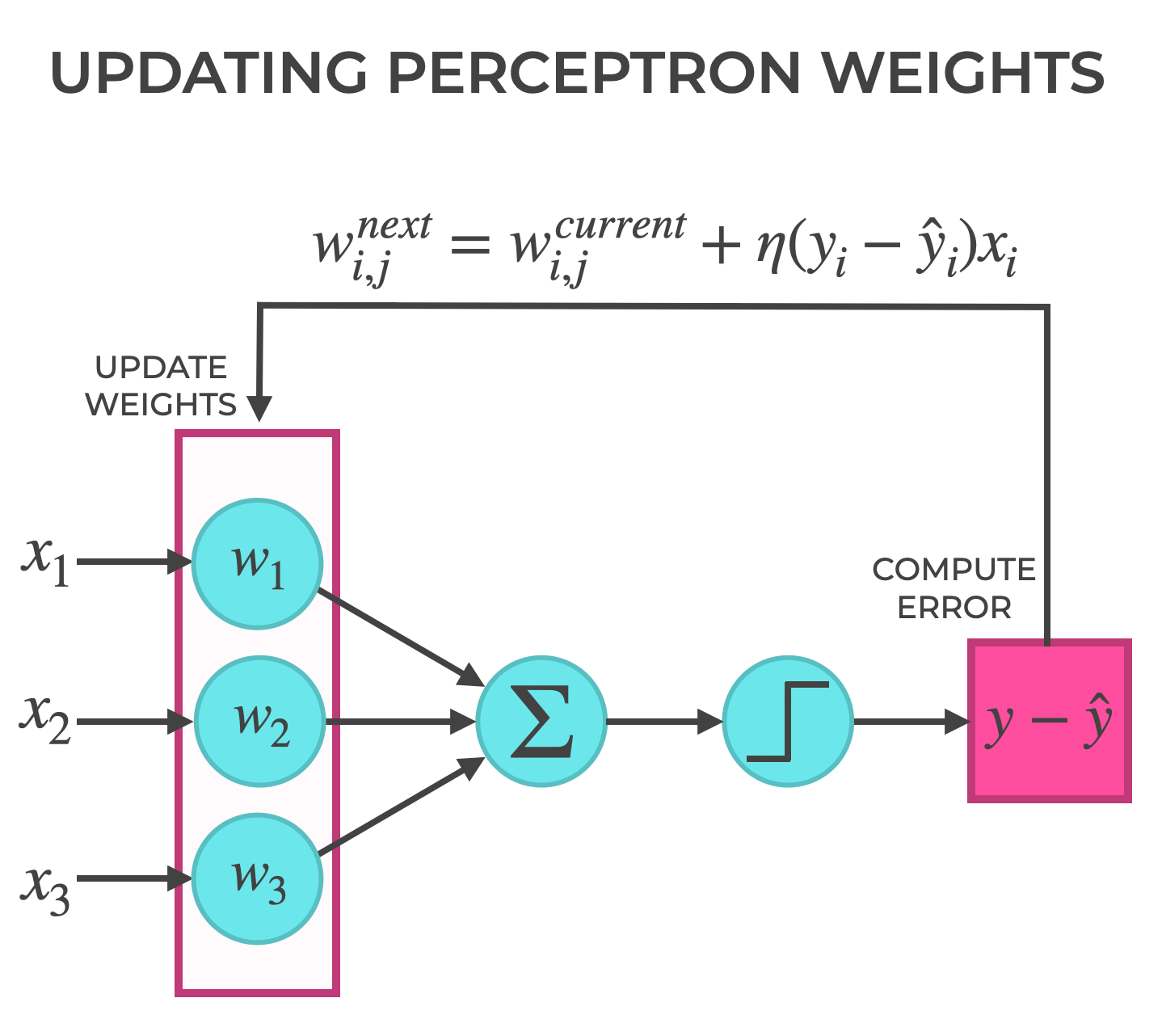
Specifically, here, we’re implementing something called the Perceptron Learning Algorithm:

(1) $\begin{equation*} w_{i,j}^{next} = w_{i,j}^{current} +\eta(y_i - \hat{y}_i)x_i \end{equation*}$

The Perceptron learning algorithm is an ALGORITHM that (surprise, surprise) allows our weights to learn how to solve a problem.

More specifically, it’s an algorithm for adjusting the weights of the Perceptron to help it solve our task better and better as we run the algorithm over many iterations.

I’m sure that looks complicated, so let’s break it down:

$w_{i,j}^{current}$ is the set of weights for the current iteration.
$w_{i,j}^{next}$ is the set of weights for the next iteration. Remember, we’re using the Perceptron Learning Algorithm to update and improve the weight values.
$\eta$ is the learning rate. This is an important tuning parameter that dictates how quickly the model updates the weights (i.e., does it make big changes or small changes?)
$y_i$ is the target output of dataset that we use during training. When we train our model, it’s the true value that we use as a point of reference during learning.
$\hat{y}_i$ is the actual output of the Perceptron. When we calculate $y_i - \hat{y}_i$ during training, we’re trying to find out how different the actual output is from the “true” value from our training dataset.
Finally, $x_i$ is the vector of input values

Jesus.

I’m exhausted just explaining all of that.

So what does all of this DO?

The Perceptron Learning Algorithm takes the output of the model, $\hat{y}_i$ , compares to the true output that we should expect, $y_i$ , and uses that information, along with the learning rate, $\eta$ , and input values, $x_i$ , to compute adjustments to the current weights, $w_{i,j}^{current}$ . We then update the current weights with the computed weight adjustment to produce the new output weights, $w_{i,j}^{next}$ .

Got it?

THAT is how the perceptron learns. It’s just applying an algorithm to update the Perceptron weights.

Model Fitting Code

Now that I’ve explained that, we’re ready to look at the code for the fit() method.

We’re going to call this fit() because that’s the convention for the Python machine learning toolkit, scikit learn.

There are two inputs:

features
targets

When we call the method, features will be a 2 dimensional Numpy array that contains the features of our training set. These are otherwise called the X_train values.

The targets input will be the target y values that we use during training (the “true” y values in our training dataset).

    def fit(self, features, targets):
        n_examples, n_features = features.shape
        
        # possibly change these
        self.weights = np.random.uniform(size = n_features, low = -0.5, high = 0.5)
        self.bias = np.random.uniform(low = -0.5, high = 0.5)
        
        for _ in range(self.n_iterations):
            for example_index, example_features in enumerate(features):
                net_input = np.dot(example_features, self.weights) + self.bias
                y_predicted = self.activation_function(net_input)
                self._update_weights(example_features, targets[example_index], y_predicted)

Notice that the first thing we do inside the method is get the shape of features. Remember: features will be a Numpy array and we can use the shape attribute to get the number of rows and columns. That’s exactly what were doing with the line n_examples, n_features = features.shape. We’re passing the number of rows to n_examples and passing the number of columns to n_features.

After that, we’re using Numpy random rand to set both the weights and the bias term of our Perceptron (remember, we defined self.weights in .__init__()). As you might expect, this sets the weights and bias term to random values, although we could initialize the values to 0 or use a different initialization scheme. For our purposes, random values is probably OK, but for more advanced neural network types (like deep networks), weight initialization is an important factor in network performance, and you need to choose the right initialization scheme depending on your exact network architecture and task.

Next is the really important part of our fit() method, the for loop that iterates through our training data and updates the Perceptron weights.

The beginning of the block, for _ in range(self.n_iterations) just says that we’re going to execute the following code for a number of iterations equal to n_iterations. The number of iterations is a parameter that we can change manually, but a reasonable number is something like 1000 to 2000.

The second, nested for loop is where we iterate through our training data. example_features is the feature data for a given example (i.e., row of data). example_index the the row number (the index of the row), which starts at 0. We can use enumerate() to retrieve both the row number and the row data from our the feature data stored in the Numpy array called features.

On the next line, we’re computing the net input: net_input = np.dot(example_features, self.weights) + self.bias. This is the value of the weights for the current row, times the input feature data, plus the bias term.

Next, we pass net_input to our activation function with the code self.activation_function(net_input). This checks if the net input meets our threshold, and returns a 0 or 1, according to the activation_function() method that we defined previously.

The output of activation_function() is the output of the perceptron. We’re calling that y_predicted, because it’s the y value that the Perceptron predicts for that row, for the current iteration, given the weights, biases, and inputs.

But remember what I mentioned about perceptron learning previously. We compare the predicted value to the “true” value, and then use the difference (along with the learning rate and input values) to update the weights … to improve the weights so that the Perceptron will make a better prediction on the next iteration.

And that’s what happens on the next line of code … we pass y_predicted to our method called _update_weights().

Update Weights Method

Here’s our code for updating the weights of our Perceptron, during model training:

    def _update_weights(self, example_features, y_actual, y_predicted):
        error = y_actual - y_predicted
        weight_correction = self.learning_rate * error
        self.weights = self.weights + weight_correction * example_features
        self.bias = self.bias + weight_correction

The _update_weights() method is actually where we implement the Perceptron Learning Algorithm:

(2) $\begin{equation*} w_{i,j}^{next} = w_{i,j}^{current} +\eta(y_i - \hat{y}_i)x_i \end{equation*}$

In this function, we’re computing the error as y_actual - y_predicted (and remember that y_predicted was computed as one of the last steps in the .fit() method discussed previously).

The weight_correction term is error multiplied by the learning rate (in the Perceptron Learning algorithm, this is $\eta(y_i - \hat{y}_i)$ ).

Then we update the weights as self.weights = self.weights + weight_correction * example_features.

… and we update the bias as self.bias = self.bias + weight_correction.

Remember: updating self.weights is the part of the Perceptron Learning Algorithm where we take the weights as they were before update, $w_{i,j}^{current}$ , and update them to new values, $w_{i,j}^{next}$ , that enable the model to work better.

The new outputs are the “corrected” weights and biases.

Again: this code is just an implementation of the Perceptron Learning Algorithm that updates the weights and bias terms so that the Perceptron can “learn” as we expose it to data and try to correct the errors in the predictions.

Predict Method

Finally, we have a .predict() method. We’ve used this name because it literally makes predictions when we give it new examples, but also because it’s consistent with the Scikit Learn machine learning API for Python.

    def predict(self, features):
        net_input = np.dot(features, self.weights) + self.bias
        y_predicted = self.activation_function(net_input)
        return y_predicted

Notice that .predict() takes new data from the features array as an input. When we call the method, this input data is commonly called X_test. This should be an input Numpy array with rows of feature data.

Once we input that feature data, we compute the net input as the dot product of input feature values and Perceptron weights plus the bias term. That’s the net_input, which we then pass to our activation function (which we discussed previously).

The output of the method is y_predicted, which is a binary output, either 0 or 1.

This code is almost identical to the code that we used in the .fit() method, except here, we return y_predicted when we call the method. The .fit() method only updates the weights, but .predict() makes predictions with the Perceptron after the Perceptron has been trained with our training data.

Concluding Remarks

So that’s it!

That’s how you create a perceptron in Python, from scratch.

As you can see, there’s a lot here.

And to do this, you really need to know a fair amount about:

Numpy arrays, and how they’re structured.
Numpy functions, for manipulating Numpy data (such as np.dot and np.where).
The Perceptron Learning Algorithm.
Python essentials like variable assignment, tuple unpacking, loops, enumerate, and more.
The basics of class and method design in Python.
Best practices of “clean code” programming.

If you’re confused at any point during this tutorial, it’s probably because you need more knowledge and intuition about one of the areas mentioned above.

And being confused is okay! This is sort of a complicated topic, and there’s a lot of moving parts.

As always, my recommendation is focus on foundations, master essential skills and concepts, and then ramp up the complexity.

In a future blog post, I’m going to execute this code and show you what it looks like when we use our perceptron to classify a binary dataset.

Leave Your Questions and Comments Below

Do you have other questions about our Python Perceptron?

Is there something that’s confusing?

Do you wish that I did something else?

I want to hear from you.

Leave your questions and comments in the comments section at the bottom of the page.