This tutorial will show you how to add ggplot titles to data visualizations in R.
It will show you step by step how to add titles to your ggplot2 plots. We’ll talk about how to:
- add an overall plot title to a ggplot plot
- add a subtitle in ggplot
- change the x and y axis titles in ggplot
- add a plot caption in ggplot
To add titles in ggplot, you need to understand how ggplot2 works
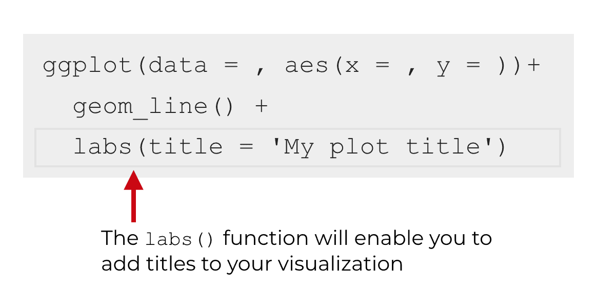
There are several ways to add titles to ggplot2 visualizations, but the primary way to add titles in ggplot2 is by using the labs() function.
Later in this post, I’ll explain the syntax of the labs() function and show you some examples.
But first, I want to give you a quick review of ggplot2.
A quick review of ggplot2
If you’re reading this blog post, you probably know a little bit about ggplot2.
But to understand how to add titles in ggplot2, it helps to really understand how the ggplot2 system works. With that in mind, to make sure you have the background that you need, I’m going to quickly explain how ggplot2 works.
Note: If you want to skip this section and move straight to the section about ggplot2 titles, you can click on this link to skip ahead.
For a more in-depth explanation, I recommend that you read our ggplot2 tutorial.
ggplot2 is a toolkit for data visualization in R
ggplot2 is a package for the R programming language that focuses on data visualization. It gives you a toolkit for creating data visualizations in R.
Keep in mind, ggplot2 is the name of the actual package, but many people use the words ggplot and ggplot2 interchangeably. So, when I’m talking about the package, sometimes write “ggplot” and sometimes write “ggplot2.” For example, in this post, we’re talking about how to add a “ggplot title” … ggplot is just a nickname for “ggplot2”. Remember, people use the terms interchangeably.
ggplot2 has different functions for different tasks
The ggplot2 visualization package is structured in a highly modular way.
What I mean by this is that the package has many different functions, and each function “does one thing.”
So there’s one function to initiate a plot. There’s one function to add lines to a plot. There is a different function to add titles. Etcetera.
So for example, if you want to create a line chart, you’ll use the ggplot() function to initiate plotting.
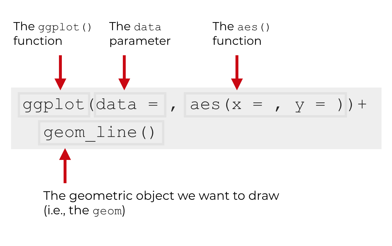
Inside of the ggplot() function, there’s the aes() function, which enables you to specify which variables should go on which axes of chart.
There’s a separate function, geom_line(), which actually draws the lines.
And if you want to add a title to your plot, there’s a separate function for that too.
Essentially, ggplot2 has discrete functions for almost everything you need to do to create a data visualization.
I want to explain that to you, because this is different than many other programming languages. Data visualization in other programing langues (like Python) is not based on discrete functions in this way.
I’m pointing out the modular design of ggplot2 because it’s somewhat relevant to how we add titles to a ggplot2 visualization.
The labs function adds ggplot titles
As I just mentioned, if you want to add a title to your ggplot2 plot, you need to call an additional function.
As it turns out, there’s actually a few functions that enable you to add titles to your plot. The ggtitle() function enables you to add an overall plot title. The xlab() function adds an x-axis title and the ylab() function enables you to add a y-axis title.
However, the labs() function can do all of these.
In the rest of this blog post, we’ll be using the labs function to add titles to our ggplot2 plots.
The syntax of the ggplot labs function
Let’s take a look at the syntax of the labs function and how it works.
As I mentioned previously in this tutorial, the ggplot2 system is highly modular.
What this means is that in order to add a title to a ggplot2 plot, you first need to create the plot itself, and then use the labs function after that.
So for example, let’s say that you want to add a title to a line chart.
You’ll first use the ggplot() function, the aes() function, and geom_line() to create a line chart.
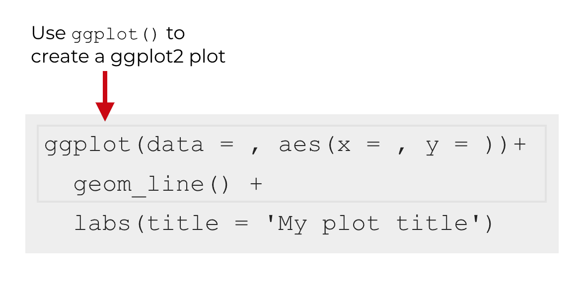
After you create your plot with ggplot(), you can add the syntax for the labs function after that:
Notice as well that in this particular example, there is a ‘+‘ after geom_line().
You always need to use a plus symbol (‘+‘) when you add a title using the labs function. This is part of the modular system of ggplot2. You’ll call the ggplot() function, and whenever you call an additional function after ggplot() to modify the plot, you’ll almost always need to use the plus sign.
A detailed explanation of the labs function
Now that you’ve seen where the ggplot labs function fits into the overall ggplot2 system, let’s take a closer look at the internal syntax of the labs function.
When you use the function, you’ll simply call the function by typing labs(), just as I explained above.
But inside of the labs function, there are several parameters that enable you to modify different parts of the plot.
Let’s take a look at each of those parameters, so you know what each one does.
The parameters of the ggplot labs function
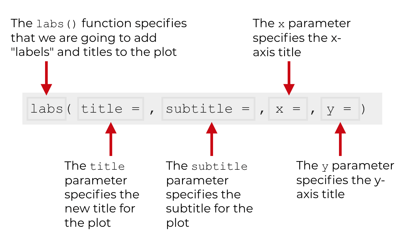
There are 5 main parameters that you should know about for the labs function:
titlesubtitlexycaption
There are also a few others (like tag), but the 5 listed above are the ones you’ll probably really use.
Importantly, each of those parameters controls a different title (AKA, “label”) of a ggplot visualization, as seen here:
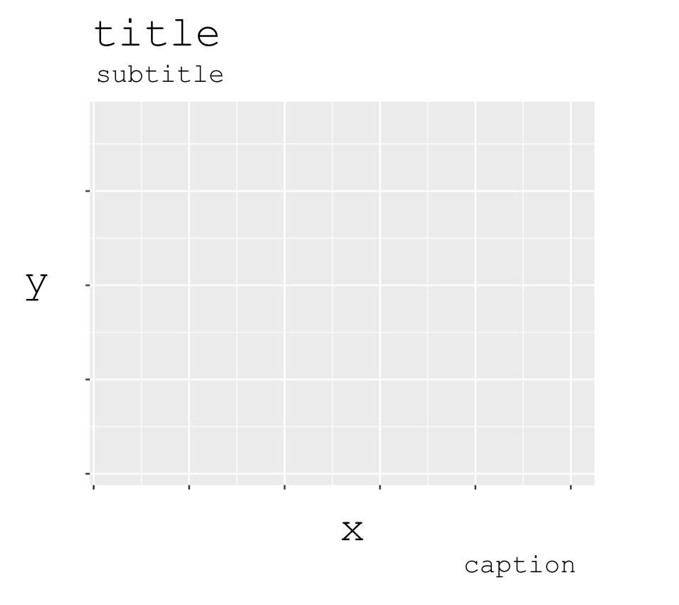
So essentially, you use the parameters to add titles or labels to specific parts of a ggplot visualization.
Let’s quickly examine each parameter.
title
The title parameter adds an overall plot title at the top of the visualization.
subtitle
The subtitle parameter adds a subtitle underneath the plot title.
x
The x parameter adds an x-axis title along the x-axis, at the bottom of the plot.
y
The y parameter adds a y-axis title along the y-axis, along the left hand side of the plot.
caption
The caption parameter adds a small plot caption at the bottom of the plot.
We will typically use this to add a small note about the plot or about the data.
These are the essential parameters of the ggplot labs function.
They’re pretty easy to use, but as always, it’s best to see how they work with real examples.
With that in mind, now let’s take a look at how to use the labs function to add labels and titles to different parts of a ggplot2 chart.
Examples: changing ggplot titles
Here in this examples section, I’ll show you simple, concrete examples of how to use the ggplot labs function to add titles.
Load and install the tidyverse package
But before you can run the code and work with these examples, you’ll need to install and load the tidyverse package.
Keep in mind that we’ll primarily be working with the ggplot2 package. However, the tidyverse package actually includes ggplot2. When you install and load tidyverse, ggplot2 will automatically be installed and loaded as well. We need to install the tidyverse because we’ll need some other tools from the tidyverse package to get our dataset.
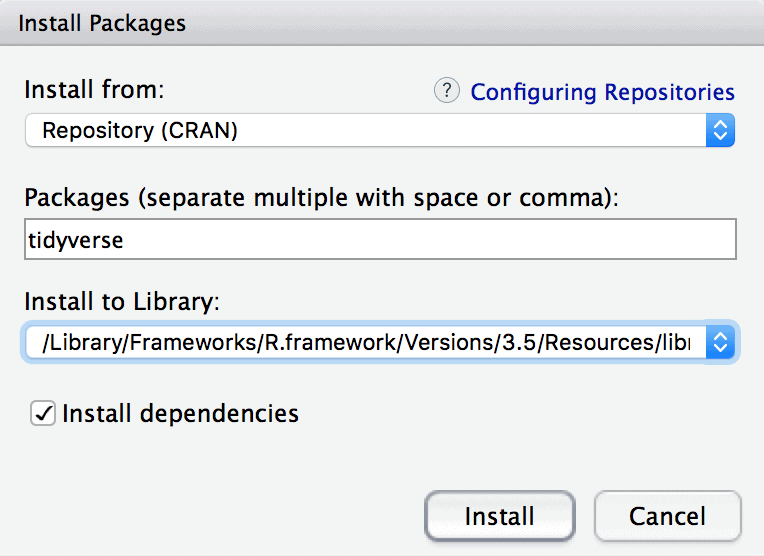
So if you haven’t already done so, install the tidyverse package.
You can install the tidyverse package in RStudio by going to the “Tools” menu, and selecting Tools >> Install Packages. This will bring up a message box that will enable you to install the package:
After you’ve installed the tidyverse package, you can load it with the library() function as follows:
library(tidyverse)
Just type that into your program and you should be ready to go.
Get dataset
Next, you’re going to need to get the data that we’ll be working with.
In the following examples, we’ll be working with some data of Tesla’s stock price.
The dataset is contained in a .csv file and is located at a specific webpage.
You’ll need to get that data and import it into R as an R data frame.
To do this, you’ll need to use the read_csv() function from the readr package. (Note that the readr package is one of the packages from the tidyverse package.)
The code to import the data into a dataframe is as follows:
# IMPORT DATA INTO R
tsla_stock_metrics <- read_csv("https://www.sharpsightlabs.com/datasets/TSLA_start-to-2018-10-26_CLEAN.csv")
After you run that code, you'll have a dataframe called tsla_stock_metrics.
As you should always do when you import data and begin working with it, you should inspect the data.
Quickly, let's print out the data to take a look:
print(tsla_stock_metrics)
Which will print out the following:
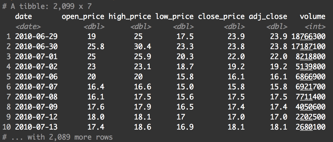
As you can see, there are several variables in this dataframe. We're primarily going to be working with the date and close_price variables.
Create a simple line chart with ggplot2
Now that we have our dataset, we can use ggplot to create a data visualization.
Remember from earlier in this tutorial: before we add a title to a plot, we must first create the plot itself.
Here, we're going to make a simple line chart.
ggplot(data = tsla_stock_metrics, aes(x = date, y = close_price)) +
  geom_line()
This code produces the following output:

Since this blog post is really about titles and not about the ggplot line chart, I'm not going to explain the code.
If you're still unfamiliar with how to create a line chart with ggplot2, you can read our detailed tutorial about ggplot line charts.
Essentially though, this is a very basic line chart made with ggplot2. There's no real formatting done on this, and this chart lacks titles.
We can use this code as a foundation to build on.
... we're going to add titles.
Add a plot title in ggplot
Ok. Now we're ready to start adding titles.
Here, we're going to add an overall plot title by using the title parameter inside of the labs() function:
ggplot(data = tsla_stock_metrics, aes(x = date, y = close_price)) +
  geom_line() +
  labs(title = 'Tesla stock price from IPO to Oct 2018')
Which produces the following chart:
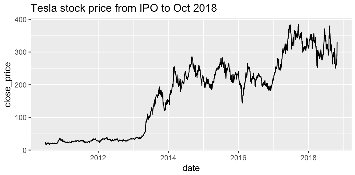
Notice that there's a title at the top of the chart now.
How did we do this?
We used the basic line chart code as a foundation. If you look at the code that we used to create this, the first two lines are exactly the same as the code that we used to create a line chart without a title.
But then the third line of code uses the labs() function. This is how we added the title.
It's really simple: we called the labs function, and inside of the function we used the title parameter to specify the title of the plot.
That's it. Simple!
Note that to add this third line of code, we needed to add the '+' symbol after geom_line(). As I explained earlier in this tutorial, that's how ggplot2 works. As you add more lines of code to modify and format a visualization, you need to use the '+' symbol to add those new lines to the data visualization code.
Keep in mind that this title is not formatted. Formatting plot titles is a little more complicated. I'll briefly talk more about formatting near the end of the tutorial.
Ok. Now let's add a subtitle.
Add a subtitle in ggplot
You can add a subtitle in exactly the same way that you added a title.
To add a subtitle, you can use the labs() function with the subtitle parameter. Essentially, inside of the labs() function, we'll use subtitle to specify the subtitle that we want to put underneath the title.
ggplot(data = tsla_stock_metrics, aes(x = date, y = close_price)) +
  geom_line() +
  labs(title = 'Tesla stock price from IPO to Oct 2018'
       ,subtitle = "TSLA price increased over 10x, but with substantial volatility"
       )
Which produces the following chart:
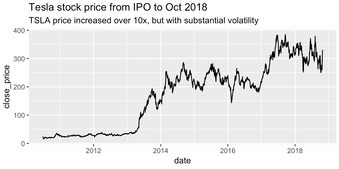
Again, this is very straightforward.
We've simply used the subtitle parameter to specify a plot subtitle.
Change the x axis title in ggplot
Now, we're going to change the x-axis title (sometimes called the 'label').
This will be very similar to the previous two examples. We're going to use the x parameter inside of the labs() function to manipulate the x-axis title:
ggplot(data = tsla_stock_metrics, aes(x = date, y = close_price)) +
  geom_line() +
  labs(x = 'Date')
Which produces the following:
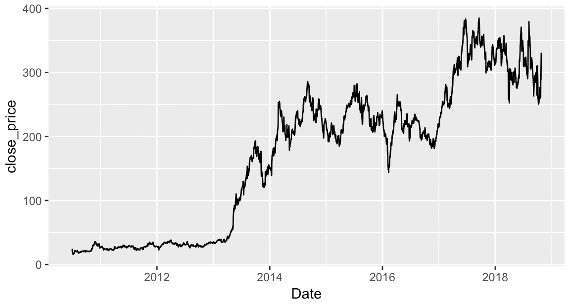
For the sake of simplicity, I've removed the title and subtitle from this chart.
Notice as well that the new title is 'Date' ... this is essentially the same as the variable name, except it is capitalized.
Now, we'll do something similar to add a y-axis title.
Change the y axis title in ggplot
Here, once again, we'll simply use the labs() function to specify the y-axis title by using the y parameter:
ggplot(data = tsla_stock_metrics, aes(x = date, y = close_price)) +
  geom_line() +
  labs(y = 'Closing Price')
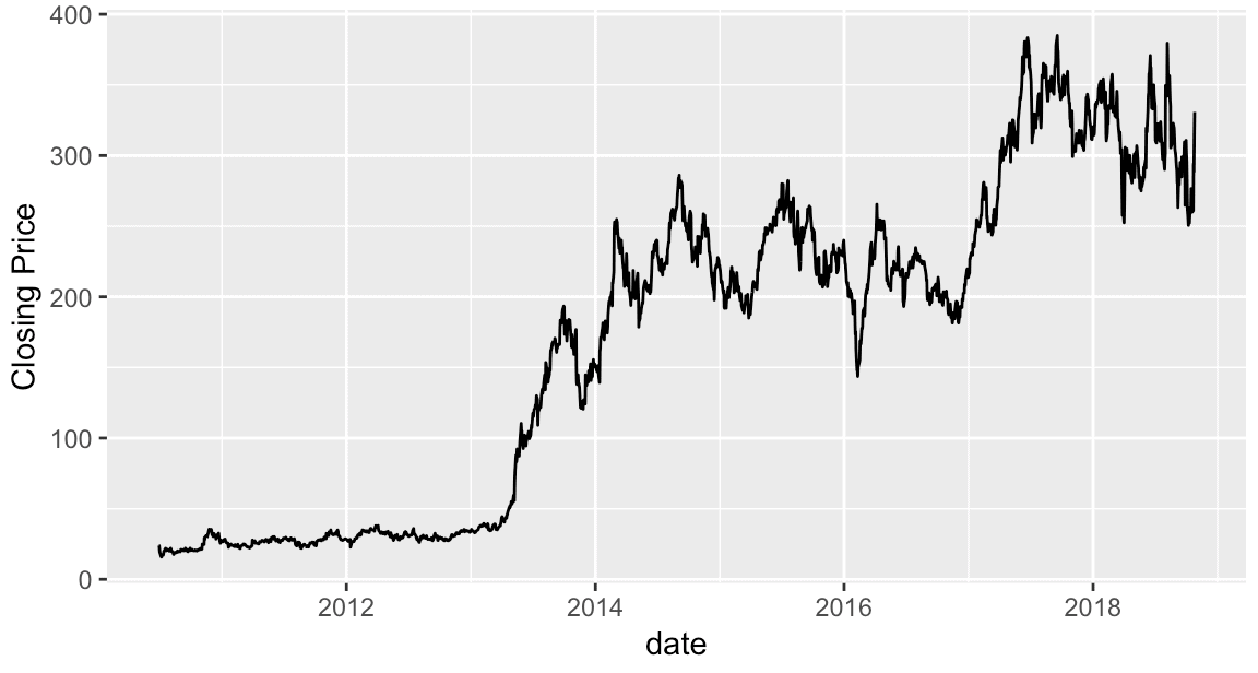
If you've already understood the previous examples, this should make sense. We've just used the y parameter inside of labs() to add a new y-axis title.
Add a plot caption in ggplot
Finally, let's add a plot caption to the bottom of the chart.
Plot captions are a good place to explain things like data sources or other notes.
Here, I'll use the caption to explain where I got the data.
Once again, we'll simply use the appropriate parameter inside of the labs function:
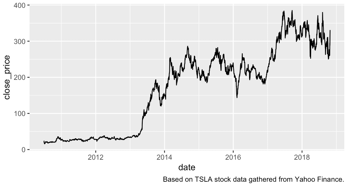
You can see the new caption at the lower right hand side of the chart, underneath the x-axis.
A quick note on formatting ggplot titles
You might have noticed that the titles for our examples are not formatted.
This is because the labs() function only allows you to specify the text of your ggplot titles. It does NOT allow you to specify the formatting.
There are separate functions for formatting your ggplot titles.
Because this blog post is really about adding ggplot titles, not about formatting, I'm not really going to explain how to format ggplot titles. Formatting is more complicated, and it will require an entirely separate blog post.
Briefly though, to format plot titles in ggplot, you'll need to use the theme() function.
Watch out for a future blog post about formatting and ggplot themes ...
Final example: modifying several ggplot titles
Ok.
I want to show you one last example.
In this example, we're going to combine several of the separate techniques that we learned about in previous sections.
We're going to use the labs() function to add a plot title, subtitle, x-axis and y-axis titles, and a caption. We'll use the labs() function to add all of them at once.
To do this, we're going to call the labs function and set values for several different parameters. Notice that the parameters are being separated by commas inside of labs.
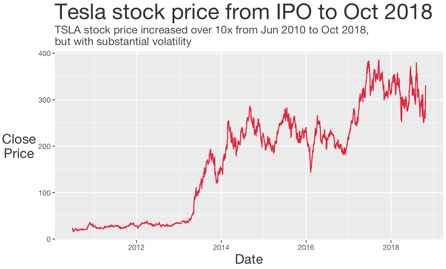
ggplot(data = tsla_stock_metrics, aes(x = date, y = close_price)) +
  geom_line(color = '#E51837', size = .6) +
  labs(title = 'Tesla stock price from IPO to Oct 2018'
       ,y = 'Close\nPrice'
       ,x = 'Date'
       ,subtitle = str_c("TSLA stock price increased over 10x from Jun 2010 to Oct 2018,\n"
                          ,"but with substantial volatility")
       ) +
  theme(text = element_text(color = "#444444", family = 'Helvetica Neue')
        ,plot.title = element_text(size = 26, color = '#333333')
        ,plot.subtitle = element_text(size = 13)
        ,axis.title = element_text(size = 16, color = '#333333')
        ,axis.title.y = element_text(angle = 0, vjust = .5)
        )
And here is the output:
Ok ...
I'll admit. There's a lot going on in this visualization.
I've used labs() to add titles, but I also made quite a few other modifications. I changed the color of the line (inside of geom_line) and I used the theme() function to make quite a few changes to the plot format.
This is a more complete and more advanced example.
Several of the techniques that I've used here are not explained in this tutorial.
Still, I want to show you what ggplot2 can really do. It's very powerful. And once you understand how it really works, it's surprisingly easy to use.
You should master the basics of ggplot2
That said, if you want to get the most out of ggplot, you need to learn more about how the ggplot syntax works.
Lucky for you ... we have plenty of tutorials here at Sharp Sight about ggplot.
For more info about ggplot, check out our tutorials on to create a ggplot bar chart, how to create a ggplot scatter plot, and how to create ggplot histograms.
We also have other tutorials about other parts of the R tidyverse: how to filter data, how add new variables to a dataframe, and how perform a variety of other data visualization and data manipulation tasks.
For more data science tutorials, sign up for our email list
Want to learn more about data science in R and data science in Python?
Sign up for our email list.
Here at Sharp Sight, we teach data science.
We regularly publish FREE articles and tutorials about data science ...
If you sign up for our email list, you'll get these tutorials delivered right to your inbox.
You'll learn about:
- ggplot2
- dplyr
- tidyr
- machine learning in R
- data science in Python
- … and more.
Want to learn data science? Sign up now.
Great Article. Am a newbie to R programming but I have found this article concise and inspirational.
From Uganda East Africa