The Best Way to Plot an ROC Curve in Python

This tutorial will show you how to plot an ROC curve in Python using the Seaborn Objects visualization package.

The tutorial is divided into sections for easy navigation, so if you need anything specific, just click on the appropriate link below.

Table of Contents:

Quick Review of ROC Curves
Setup
Create Data
Plot the ROC Curve with Seaborn Objects
Why Use Seaborn for ROC Curves
Frequently Asked Questions

A Quick Review of ROC Curves

I recently published a rather extensive article on ROC curves, but here, let’s start with a quick review of what ROC curves are.

In machine learning classification systems, ROC curves are an indispensable tool for model evaluation. In particular, we use them with binary classification (although, there are some ways to use ROC curves with multiclass classification as well).

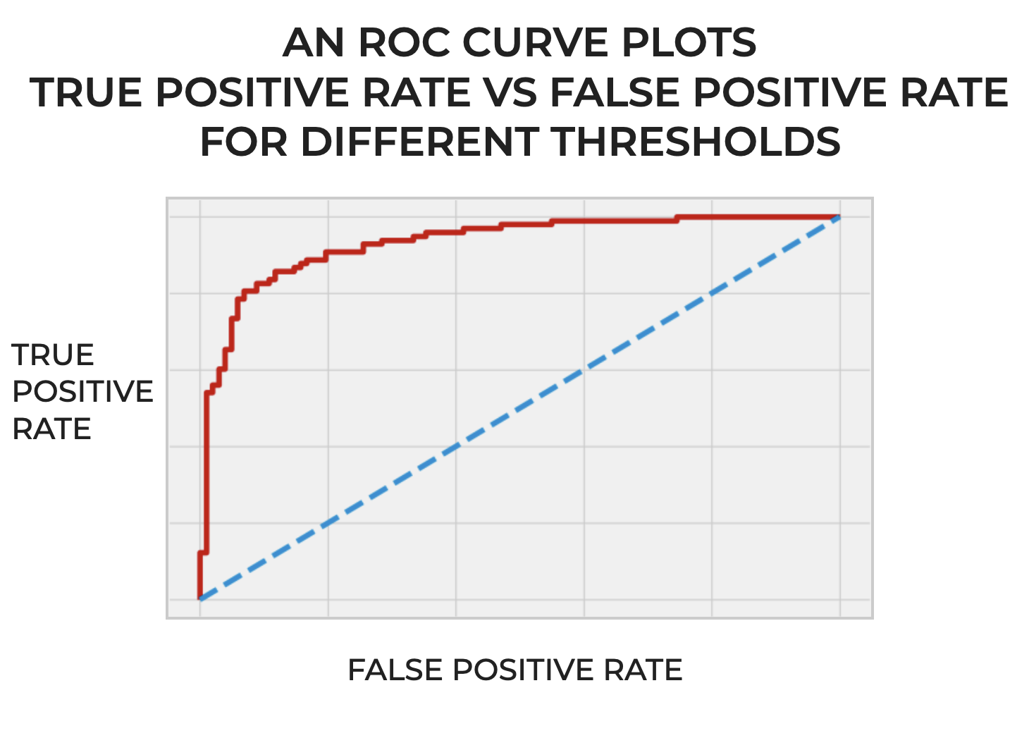
Put simply, an ROC curve visualizes the True Positive Rate and False Positive rate for a classifier, across a range of classification thresholds.

Remember: many classifiers, and probabilistic classifiers in particular, produce a “probability score” that measures the classifier’s confidence that a particular example belongs to the positive class. These classifiers compare the probability score to a threshold, and this determines which examples will be predicted as positive, and which will be predicted as negative.

Moreover, because we can move the threshold, the number of positives and negatives depends on the choice of threshold.

The ROC curves helps us understand the tradeoff between detecting True Positives and avoiding False Positives, as we change the classification threshold.

And in doing this, they ultimately illustrate the ability of a classifier to differentiate between the positive and negative for different threshold values.

Why We Need ROC Curves

Ok. So ROC curves help us visualize True Positive rate and False Positive rate.

By why do we need them exactly?

Once again: The power of ROC curves lies in their ability to depict how well a classifier distinguishes between positive and negative classes across a range of thresholds.

So in essence, they show us how the model will perform across range of threshold settings, and this in turn can help us choose the right operating point (i.e., the right threshold setting) given the goals and needs of our system.

In some systems, you might want to minimize False Positives, and want a high threshold.

In other systems, you might want to maximize True Positives, and decide to set a lower threshold.

In either case though, an ROC curve will show you the tradeoff for those metrics for your classifier, as you move the threshold. And in turn, that will help you pick the best threshold for your needs, given those tradeoffs.

Good and Bad ROC Curves

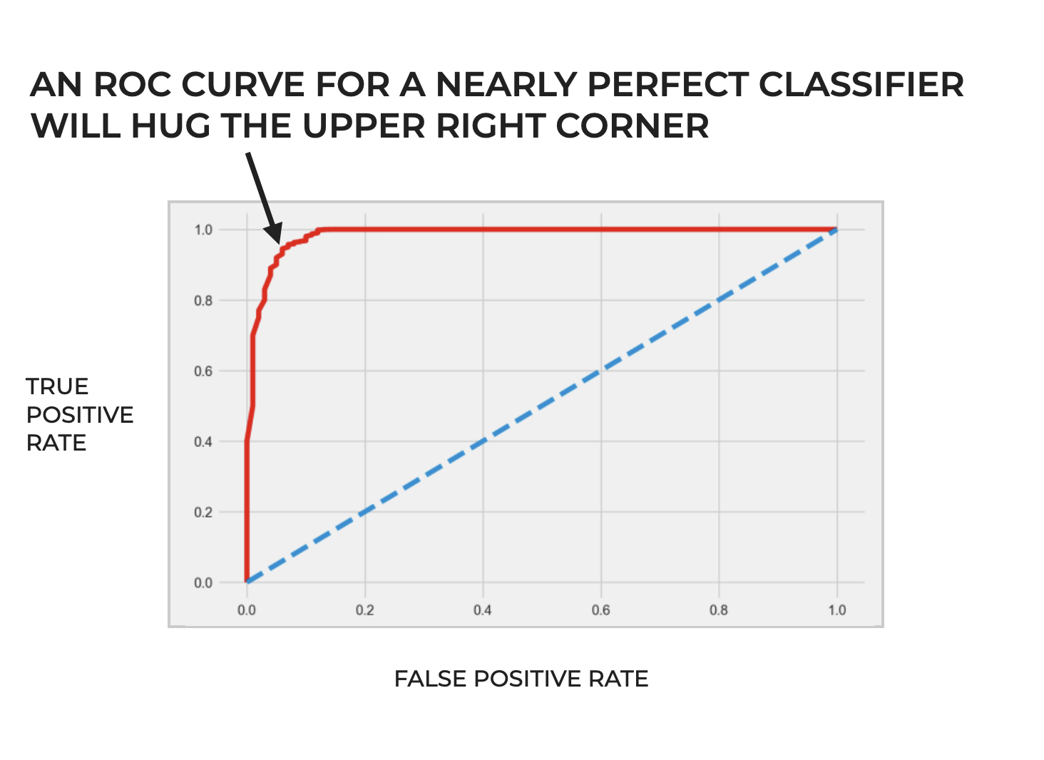
Generally speaking, a classifier that performs well will have an ROC curve that hugs the top left corner. This indicates that the model can achieve high True Positive rate and with a low False Positive rate.

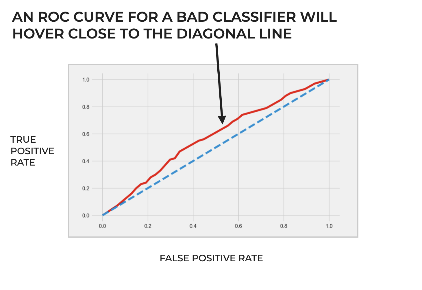
Alternatively, a classifier that performs poorly will have an ROC curve that hugs the diagonal line from the bottom left hand corner to the upper right.

To be clear though, ROC curves can be a complicated topic, and I’m leaving out some important details. For a more in-depth explanation, you should read our blog post ROC Curves, Explained.

In the rest of this blog post, I want to show you how to create an ROC curve in Python, with my favorite Python visualization package.

Plot an ROC Curve in Python using Seaborn Objects

In this tutorial, I’m going to show you how to plot an ROC curve in Python.

Specifically, we’re going to plot an ROC curve using the Seaborn Objects visualization package.

But doing that will require several steps.

We need to:

import packages
create the ROC curve data
plot the ROC curve

Let’s take those one at a time.

If you already have some ROC curve data – meaning true positive and false positive metrics – then feel free to skip to the section where we plot the ROC curve with Seaborn.

Import Packages

First, we need to import several packages.

We’re going to plot the ROC curve with the Seaborn objects system, so we obviously need to import that.

But before we plot it, we need to generate the data for the ROC curve itself, which will require several steps. Specifically, we need to:

create a classification dataset
split the data
build a classification model (in this case we’ll use logistic regression)
generate the false positive/true positive data for the ROC curve itself

That being said, we also need to import make_classification, train_test_split, LogisticRegression, and roc_curve from Scikit Learn in order to do all of those things.

# roc curve and auc
from sklearn.datasets import make_classification
from sklearn.linear_model import LogisticRegression
from sklearn.model_selection import train_test_split
from sklearn.metrics import roc_curve

import seaborn.objects as so

Make Data for ROC Curve

Next, we need to make the data for our Python ROC curve.

Remember: when we plot an ROC curve, we plot the false-positive-rate vs the true-positive-rate.

In other words, we need to generate data for false positive rate and true positive rate for a classification model.

There are many steps to this.

In this case, we need to:

create a classification dataset with sklearn make_classification
split the data with Scikit learn’s train_test_split function
build the model (in this case, we’ll build a Logistic Regression model)
predict the probabilities for the X test data, using Scikit Learn predict_proba
calculate the true positive and false positive data with the Scikit Learn roc_curve function

In the interest of brevity, and because this tutorial is about plotting an ROC curve, I’m going to refrain from explaining each step. You can click on any of the above links to understand each step.

# GENERATE CLASSIFICATIONDATASET WITH 2 CLASSES
X, y = make_classification(n_samples=1000, n_classes=2, random_state=1)


# SPLIT DATA INTO TRAIN/TEST
X_train, X_test, y_train, y_test = train_test_split(X, y, test_size=0.2, random_state=2)


# GENERATE DATA FOR 45-DEGREE LINE
noskill_probabilities = [0 for number in range(len(y_test))]


# BUILD & FIT CLASSIFICATION MODEL
my_logistic_reg = LogisticRegression()
my_logistic_reg.fit(X_train, y_train)


# PREDICT PROBABILITIES FOR TEST SET
probabilities_logistic_reg = my_logistic_reg.predict_proba(X_test)


# KEEP PROBABILITIES FOR ONLY THE POSITIVE OUTCOME
probabilities_logistic_posclass = probabilities_logistic_reg[:, 1]

# CALCULATE DATA FOR HORIZONTAL LINE
falseposrate_noskill, trueposrate_noskill, _ = roc_curve(y_test, noskill_probabilities)

# CALCULATE DATA FOR ROC CURVE (Logistic Regression Model)
falseposrate_logistic, trueposrate_logistic, _ = roc_curve(y_test, probabilities_logistic_posclass)

Once you run this code, you’ll have the true positive data (trueposrate_logistic) and false positive data (falseposrate_logistic) that you need for the Python ROC curve.

Plot the ROC Curve with Seaborn Objects

Here, we’re going to use Seaborn to plot the our Python ROC curve.

Remember: when we plot an ROC curve, we plot the false positive rate vs the true positive rate.

That means here, we’re going to plot falseposrate_logistic vs trueposrate_logistic.

And to do this, we’ll use the Seaborn Objects visualization system to create a line chart from our true positive/false positive data.

Let’s run the code, and then I’ll explain.

# PLOT: SEABORN OBJECTS
(so.Plot()
   .add(so.Line(color = 'red'),x =falseposrate_logistic, y = trueposrate_logistic)
   .add(so.Line(color = 'blue',linestyle = 'dashed'),x = falseposrate_noskill, y = trueposrate_noskill)
   .layout(size = (8,5))
)

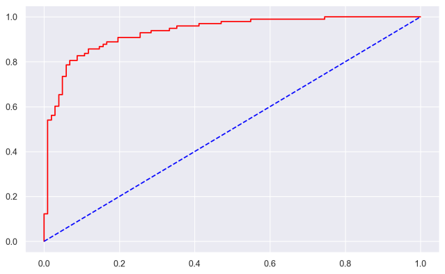
OUT:

Explanation

So what did we do here?

Here, we’ve used the Seaborn Objects system to plot both the ROC curve for the model (in red) as well as the diagonal reference line (in blue).

Syntactically, we’re using the Seaborn Objects .add() method to add each line.

The first call to .add() adds the red ROC curve, and the second call to .add() adds the dashed blue reference line.

If you want to learn more about the line charts with Seaborn Objects, you should read our tutorial about Seaborn Objects line plots.

Closing Note: Use Seaborn for ML Visualization

One last closing note.

I recommend using Seaborn for almost all of your data visualization in Python.

And in particular, I recommend it for your data visualization tasks related to machine learning in Python.

The new Seaborn Objects system has a very easy-to-use syntax.

It’s much easier to use than Matplotlib.

It’s easier to use than Plotly.

And it’s extremely powerful, one you know how to use it.

I’ve started doing 98% of my visualization with Seaborn Objects, and I recommend that you do the same.

So it’s not only great for making an ROC curve in Python machine learning, but also a variety of other ML visualizations.

Leave your other questions in the comments below

Do you still have questions about how to make an ROC curve in Python?

Leave your questions in the comments section below.

For more machine learning tutorials, sign up for our email list

This tutorials should have shown you how make an ROC curve in Python using Seaborn.

But if you want to master machine learning in Python, there’s a lot more to learn.

If you want free tutorials about machine learning in Python, then sign up for our email list.

When you sign up, you’ll get free tutorials on:

Scikit learn
Machine learning
Deep learning
NumPy
Pandas
… and more.

So if you want to master machine learning, deep learning, and AI in Python, then sign up now.