Binary Classification, Explained

Binary classification stands as a fundamental concept of machine learning, serving as the cornerstone for many predictive modeling tasks.

At its core, binary classification involves categorizing data into two distinct groups based on specific criteria, a process akin to making a ‘yes or no’ decision.

This simplicity conceals its broad usefulness, in tasks ranging from email spam detection to medical diagnosis.

This blog post aims to demystify binary classification, clearly explaining what it is, key concepts, and a few real-world examples.

If you need something specific, you can click on any of these following links:

Table of Contents:

A Quick Review of Machine Learning and Classification
What is ‘Binary’ Classification?
An Example of Binary Classification
Common Binary Classification Algorithms
Binary Classification Metrics

Whether you’re a beginner in data science or seeking to refresh your knowledge, this article will offer a clear and concise understanding of binary classification and its pivotal role in machine learning.

Let’s get to it.

A Quick Review of Machine Learning

Machine learning is a subset of artificial intelligence that enables computers to learn from data and subsequently make decisions based on what it learns.

Unlike traditional programming, where a human explicitly codes how the program works (typically as strict if-then rules), machine learning algorithms learn patterns as they are exposed to data examples. They learn how to operate as opposed to being explicitly directed with if/then code. So, using statistics, algorithms, and innovative computer science techniques, machine learning “teaches” computers how to perform tasks and improve performance on those tasks.

At the heart of machine learning is the concept of a ‘model’ – a mathematical representation of a real-world process. By feeding data to the algorithms at the core of these models, we can train them to make predictions or classify data. The training process adjusts the model’s “parameters” until it can accurately perform the task it is being trained to do.

Types of Machine Learning

There are three main types of machine learning: supervised learning, unsupervised learning, and reinforcement learning.

Although unsupervised and reinforcement learning are important, for the purposes of our discussion about classification, the most important is supervised learning.

Supervised learning involves training a model on a labeled dataset, where the desired outcome is known. Supervised learning literally shows a machine learning algorithm “examples” where the answer is already known, so the algorithm can learn the patterns associated with generating the correct answer.

We can further break out supervised learning into different types of tasks, like regression and classification.

In fact, in supervised learning, classification is one of the most important and most common task.

Classification involves categorizing data into predefined classes, like spam and not spam or cat and non cat. It’s important to remember: in classification, we already have a set of pre-defined classes that are possible. The purpose of a classification system is to learn how to predict the correct output class (from the pre defined set of possible classes), based on input data.

And that brings us to binary classification, which is a special case of classification more broadly.

What is ‘Binary’ Classification

Binary classification is a specific type of classification task in machine learning where the goal is to categorize incoming examples into one of two distinct groups … thus the use of the term ‘binary.’

So whereas classification generally chooses (i.e., predicts) the appropriate label from a set of possible labels, binary classification chooses the appropriate label from only two possible labels.

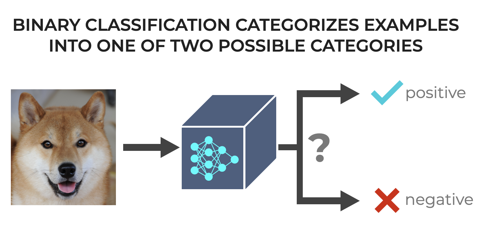
It’s about making a choice between two options, often labeled as 0 and 1, true and false, or yes and no, and perhaps most importantly positive and negative (which I’ll discuss more in a little bit)

Although binary classification can be used in a variety of ways, this form of classification is particularly useful in scenarios where we’re detecting the presence or absence of something, such as detecting fraudulent transactions (fraud or no fraud) or diagnosing a medical condition (disease present or not present).

The simplicity of binary classification lies in its focus on just two categories. Furthermore, more complex classification tasks – such as multiclass classification, which has more than two classes – typically have foundations that built are built on binary classification. That is, to understand multiclass classification concepts, you frequently need to understand binary classification first.

So understanding binary classification not only gives you a powerful toolkit for tackling many real world problems (since many real-world problems are naturally binary), mastering binary classification also provides a solid foundation for tackling more complex and nuanced machine learning problems.

A Simple Example of a Binary Classifier

Ok.

Let me show you a simple example.

This is a common example that I use in many of my blog posts, because it’s easy for most people to understand.

It’s called, The Cat Detector.

The Cat Detector is simple.

It detects cats.

You feed it an image, and it predicts if that image is a cat or not a cat.

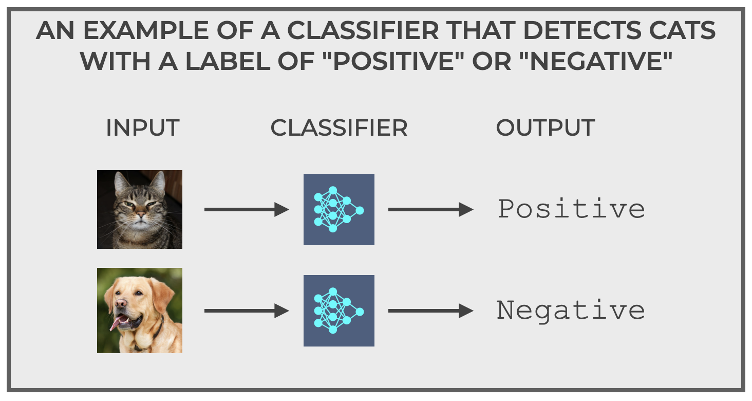
Specifically, for the purposes of this example, the two possible output labels are positive and negative. These labels are very common labels in binary classification systems, because they’re general terms that also conform to the names of common (and important) binary classification metrics like True Positive, True Negative, False Positive, and False Negative.

And in turn, those quantities (TP, TN, FP, and FN) are used in almost all of our important binary classification metrics, which I’ll tell you about in a moment.

But, technically, the actual labels could be cat and non cat, or even something simpler like 1 and 0.

What’s important is that we have a system that accepts input data (examples) as inputs, and subsequently outputs one of only two possible labels, which in this example, correspond to whether the image is a cat or not a cat.

Common Binary Classification Algorithms

It’s important to remember that classification is not a technique itself, but rather, classification is a task. What that means is that there are a variety of machine learning tools (i.e., algorithms) that can perform binary classification.

Let’s quickly review the most common.

Logistic Regression

Logistic regression is arguably the quintessential binary classification algorithm, as it’s often the go-to algorithm for binary classification problems.

Logistic regression is relatively simple to understand and implement, making it an ideal starting point for beginners.

Essentially, logistic regression uses an s-shaped curve to model the data.

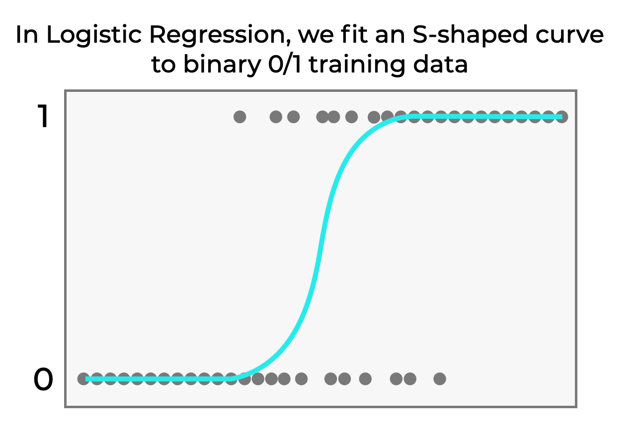
Notice that the curve trends towards 0 as x decreases, and it trends towards 1 as x increases. Because of this, we can use the logistic regression function as a way of modeling the relationship between the input variable or variables (e.g., x) and the output y variable.

Decision Trees

Decision trees are great because they are easy to visualize and (typically) easy to understand.

In their simplest form, decision trees look for “splits” in the input data.

For example:

if x is less than .05, predict 0
if x is greater than or equal to .05, predict 1

That would be a simple tree with a single split. Decision trees can have multiple splits for more complex data.

But at their core, they treat prediction as a series of if/then conditions … if A, and B, and C, then predict 0. If A and not B and not C, predict 1.

I should note that decision trees do have some problems. They are prone to overfitting.

Additionally, decision trees can also be used for multiclass classification.

But in their simplest form, they work extremely well for binary problems.

Support Vector Machines

Support Vector Machines (SVMs) are a powerful type of supervised learning algorithm used for binary classification.

At their core, SVMs attempt to find the best dividing line (or hyperplane) that separates data points of two classes.

This line is chosen to maximize the “margin” (think of the margin as the distance) between the data points of both classes, effectively creating the widest possible gap.

This approach makes SVMs particularly effective for high-dimensional problems (i.e., problems with a large number of input X variables).

By using something called the kernel trick, SVMs can handle complex nonlinear relationships, which makes them versatile and robust for various binary classification tasks.

Moreover, ability to manage overfitting – even on complex datasets – has historically made them a favorite in the machine learning community.

Deep Neural Networks

Deep Neural Networks (DNNs) are an advanced type of machine learning model inspired by the structure and function of the human brain.

They consist of several layers of interconnected artificial neurons (AKA, “nodes”) which are individually modeled after human neurons.

Deep networks excel at identifying complex, nonlinear relationships in the data. This is because typically, very layer in a deep network learns more nuanced patterns in the input data, which enables them to progressively learn more complex patterns, particularly as you add more layers.

This ability to identify complex patterns makes deep nets a powerful tool for binary classification, especially when dealing with large, high-dimensional datasets. They can capture intricate patterns that simpler models (like logistic regression) might miss.

Having said that, deep networks do tend to overfit the data, and often require very large datasets for model training. Moreover, their complexity typically makes them harder to train, tune, and understand, which can all be downsides.

Other Binary Classification Algorithms

The four algorithms that I mentioned above – logistic regression, decision trees, support vector machines, and deep neural networks – are only four of the most common among many different algorithms that we can use for binary classification.

Others include random forests and boosted trees (which are variations of decision trees); naive bayes; and k-nearest neighbors.

I must also mention that every machine learning algorithm has strengths and weaknesses.

Some are easy to use, some are difficult to use Some train fast, some train slow. Some tend to achieve high accuracy even on complex datasets, and other struggle to accurately model complex data.

And so on.

Every algorithm is like a tool in the data scientist’s toolbox. You need to know what each tool does, how it works, and when to use it.

Having said all of that, because each of the above algorithms is complex, in the interest of brevity, I’ll write more about each algorithm, how they work, and their strengths and weaknesses in another blog post.

Binary Classification Metrics and Evaluation Tools

Let’s finally do a quick review of metrics and tools that we use to evaluate binary classifiers.

The major tools and metrics that you need to know are:

confusion matrices
roc curves
precision
recall
F1 score

Let’s quickly discuss all of these.

Confusion Matrices

The confusion matrix is a simple tool that we use to visualize predictions made with a binary classifier.

For every prediction of a binary classification system, we categorize every example according to two things:

the predicted class
the actual class

So let’s go back to the Cat Detector that I described above.

When we use that binary classification system, we feed an image into the system as an input. Every picture is either a cat, or a non-cat. So every image has an actual class (positive or negative).

Then the classifier predicts what it thinks is in the image (positive for cat, negative for non-cat).

Therefore, every input example will have both a predicted class AND an actual class.

And we can subsequently group all examples into 4 buckets … two types of accurate predictions (True Positive and True Negative) as well as two types of inaccurate predictions (False Positive, and False Negative).

And furthermore, we can group all of those examples into a 2×2 matrix, like this:

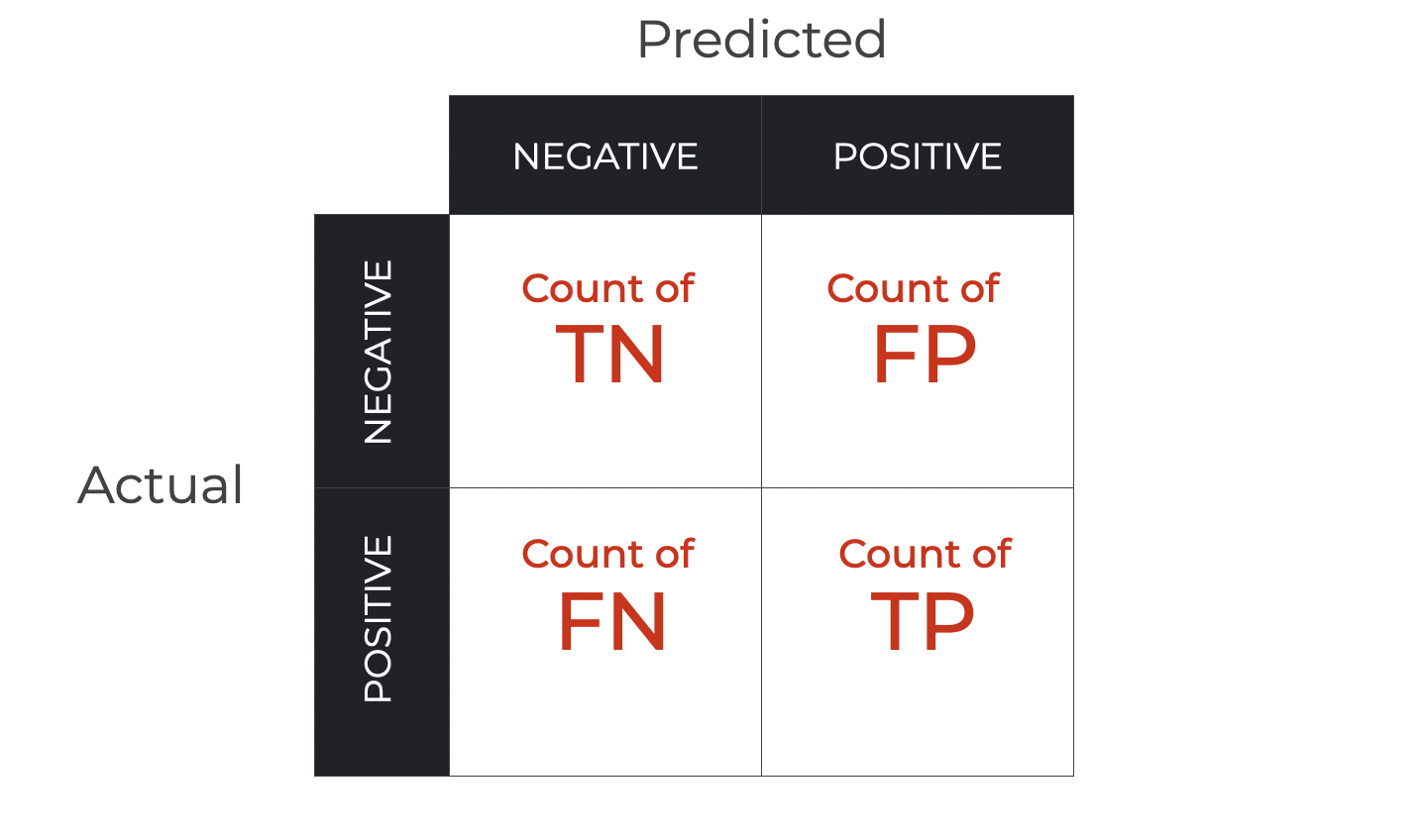
This is what we call a confusion matrix.

As you can see, it’s a simple way of organizing and visualizing the correct and incorrect predictions of a binary classifier.

And it’s arguably one of the most important tools for evaluating a binary classifier.

You can learn more about confusion matrices in our blog post: Confusion Matrices, Explained.

ROC Curves

An ROC curve is another visualization tool that we use to evaluate the performance of a binary classifier.

Put simply, an ROC curve visualizes the tradeoff between True Positives and False Negatives for different classification thresholds.

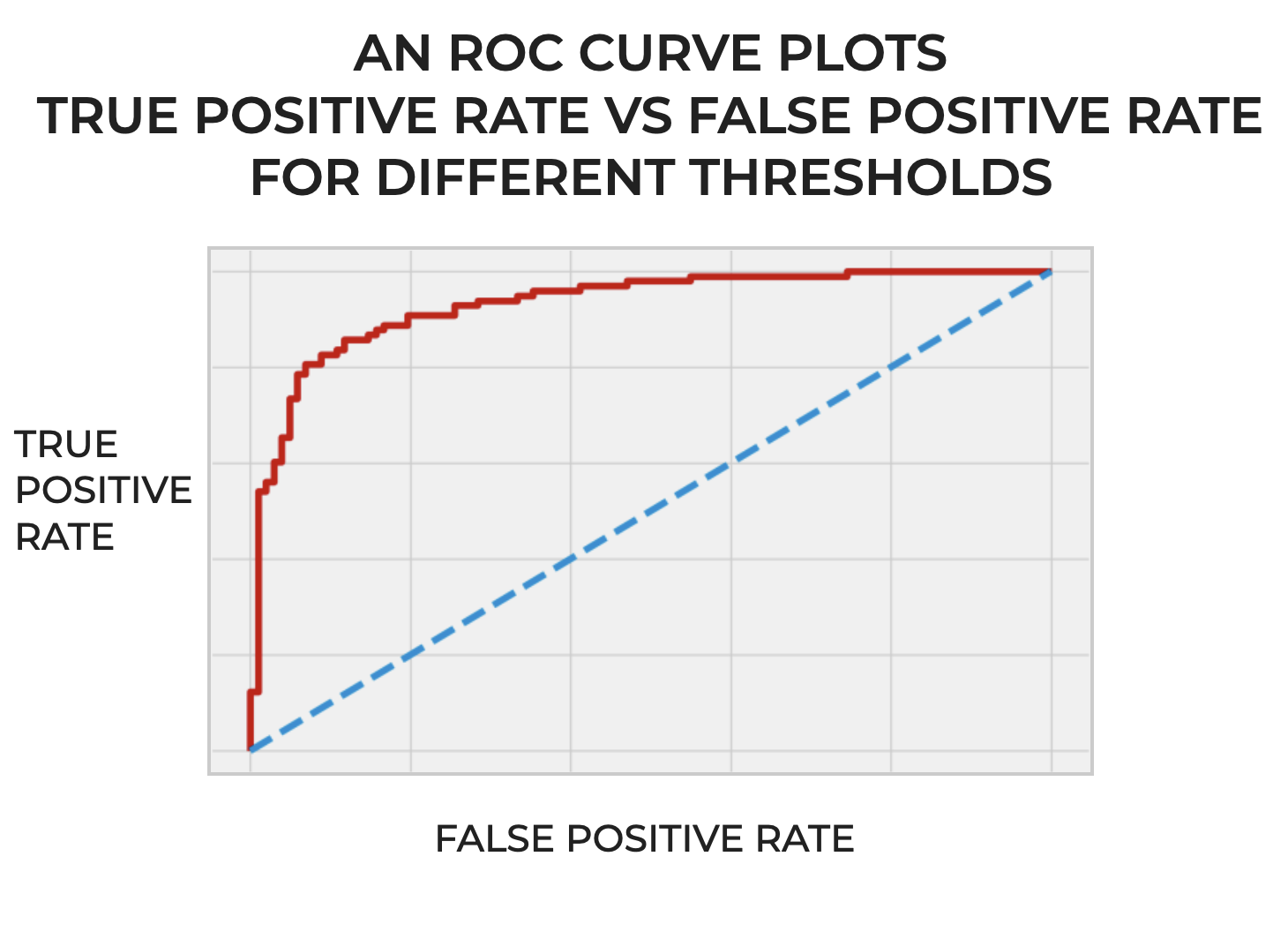
ROC curves help us visualize and understand how well a classifier predicts True Positives while also avoiding False Negatives.

Accuracy

Accuracy measures the proportion of “correct” predictions (True Positives and True Negatives) divided by all predictions.

Essentially, it measures how well the classifier predicts the positive and negative classes collectively.

We can compute accuracy as follows:

(1) $\begin{equation*} \frac{\text{TP + TN}}{\text{TP} + \text{TN} + \text{FP} + \text{FN}} \end{equation*}$

Accuracy is a good high-level metric for evaluating a binary classifier. But, it does have some problems. The biggest issue is that when a classifier makes mistakes, accuracy fails to provide information about what types of mistakes the classifier is making.

So in many cases, we might use accuracy to evaluate a classifier at a high level, but we will often also use precision, recall, F1 score, and other tools.

You can learn more about accuracy in our blog post: Classification Accuracy Explained.

Precision

Precision is a metric that quantifies the accuracy of the positive predictions made by the model.

More specifically, precision measures the proportion of positive predictions that were correct (meaning, when the model correctly predicted a positive example as positive).

We can compute precision as follows:

(2) $\begin{equation*} \frac{\text{TP}}{\text{TP} + \text{FP}} \end{equation*}$

You can learn more about precision in our blog post: Precision Explained.

Recall

Recall is like a sibling to precision.

Recall quantifies how accurately the model identifies the positive examples.

More specifically, it quantifies the proportion of actual positive examples that the model has correctly predicted as positive.

We can compute recall as follows:

(3) $\begin{equation*} \frac{\text{TP}}{\text{TP} + \text{FN}} \end{equation*}$

You can learn more about recall in our blog post: Recall Explained.

F1 Score

Finally, I’ll mention F1 score.

F1 score is like a blend of precision and recall.

We use it because precision and recall both have potential problems.

You can artificially achieve a very high precision by tuning your model to be very conservative in how it makes positive predictions (which can create a lot of False Negatives).

And you can achieve a very high recall by simply predicting every example as positive (which can create a lot of False Positives).

F1 score balances between both precision and recall, and thus avoids the issues of either too many False Negatives or too many False Positives.

To do this, F1 score computes the harmonic mean of precision and recall:

(4) $\begin{equation*} \text{F1 Score} = H(precision, recall) = \frac{2}{\frac{1}{precision} + \frac{1}{recall}} \end{equation*}$

If you plug in the equations for precision and recall that I showed earlier (and simplify the equation), you eventually get this equation in terms of True Positives, False Negatives, and False Positives:

(5) $\begin{equation*} \text{F1 Score} = \frac{\text{2TP}}{\text{2TP} + \text{FP} + \text{FN}} \end{equation*}$

Essentially, F1 score harmonizes between precision and recall. It helps us understand how well the model predicts True Positives, while simultaneously avoiding both False Positives and False Negatives.

Wrapping Up: You Need to Understand Binary Classification

Binary classification is not just a fundamental skill in machine learning. It’s a gateway to mastering machine learning and AI more broadly.

This concept, at its core, teaches us the art of making binary decision and predictions based on data, a critical skill in our data-driven world.

As many real-world problems can be framed as binary classification tasks, mastering this concept equips you with the tools to solve a wide range of practical problems, including problems in natural language processing, computer vision, banking, and more.

Additionally, binary classification serves as a building block for more complex tasks in machine learning and AI, including multi-class classification and even regression.

Ultimately, mastering binary classification opens the door to the broader landscape of machine learning and AI. It’s a critical step in becoming a proficient data scientist or AI practitioner, providing the knowledge and skills necessary to excel in this valuable field.

Leave Your Questions and Comments Below

Do you have other questions about binary classification?

Are you still confused about something, or want to learn something else about binary classifiers that I didn’t cover?

I want to hear from you.

Leave your questions and comments in the comments section at the bottom of the page.

Sign up for our email list

If you want to learn more about machine learning and AI, then sign up for our email list.

Every week, we publish free articles tutorials about various topics in machine learning, AI, and data science topics, including:

Scikit Learn
Numpy
Pandas
Machine Learning
Deep Learning
… and more

If you sign up for our email list, then we’ll deliver those free tutorials to you, direct to your inbox.