Sklearn confusion_matrix, Explained

Scikit-learn, which is affectionately known as sklearn among Python data scientists, is a Python library that offers a wide range of machine learning tools.

Among these tools is the confusion_matrix function, which is indispensable when working on classification problems.

So in this tutorial, I’ll show you how to use the sklearn confusion_matrix function.

I’ll give you a quick overview of confusion matrices, explain the syntax of sklearn confusion_matrix in particular, and I’ll show you an example of how it’s used.

Table of Contents:

• Introduction
• Syntax
• Examples
• Frequently Asked Questions

With that said, let’s dive in so you can understand this function and how to use it in your machine learning projects.

A Quick Introduction to Scikit Learn confusion_matrix

When we build a machine learning model, we need to be able to evaluate its performance.

Different model types have different tools and metrics that help us evaluate them.

And one of the most common tools for evaluating classification models is the confusion matrix.

To help you understand confusion matrices, I’m going to quickly review what classification is, and then I’ll explain how confusion matrices work conceptually.

That will set us up to look at the Scikit-learn confusion_matrix function later in the tutorial.

A quick review of classification

Classification is a type of supervised learning where we predict categorical labels on the basis of input features.

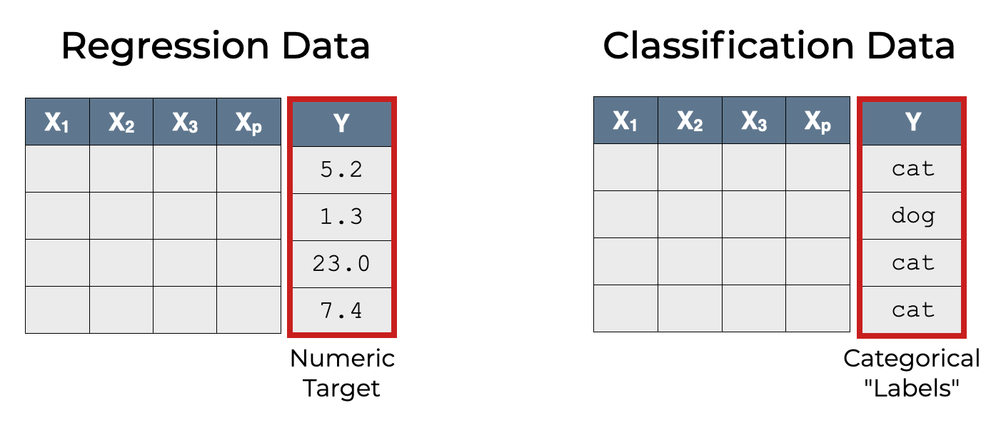
So once we train a classification model, we can use it to predict categorical labels.

A Classifier Can Make Different Types of Correct and Incorrect Predictions

Importantly, a classification model can make correct predictions and incorrect predictions.

Moreover, there are different types of correct predictions and mistakes.

To illustrate this, let’s discuss a hypothetical classification system that I’ll call The Cat Classifier.

The cat classifier does one thing: It inputs images, and labels the image as cat or not cat.

You feed it an image, and it outputs one of those two labels.

And as I already said, there are different types of correct predictions and incorrect predictions, as seen here:

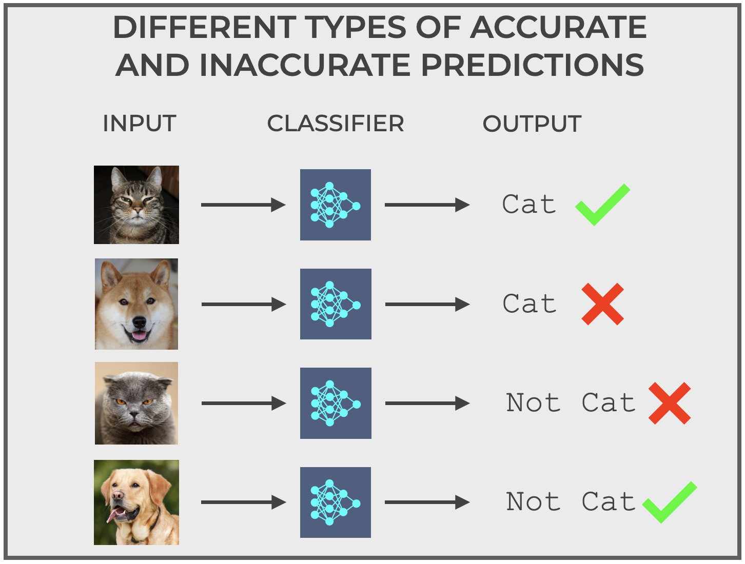
Now let’s assume that instead of the labels cat and not cat, we use the labels positive and negative instead (positive if the Cat Classifier thinks the image is a cat, and negative if it thinks its not a cat).

When the model makes a prediction, there are collectively 4 different types of correct and incorrect predictions:

• True Positive: Correctly predicts positive when the image is actually a cat
• True Negative: Correctly predicts negative when the image is not a cat
• False Positive: Incorrectly predicts positive when the image is not a cat
• False Negative: Incorrectly predicts negative when the image is actually a cat

A Confusion Matrix Visualizes Correct and Incorrect Predictions for Classification Models

A confusion matrix is a visual tool for organizing these types of correct and incorrect predictions.

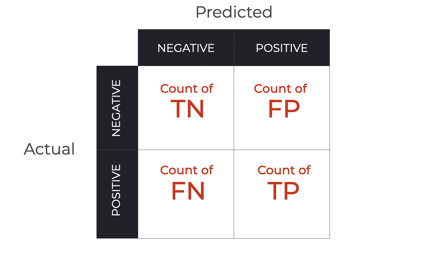
Or more accurately, it’s a way of counting the number of true positives, true negatives, false positives, and false negatives, and organizing them into a grid. This grid enables us to understand the performance of a classifier, as well as the types of mistakes it is making.

(For a more detailed description of confusion matrices, please read our recent blog post titled Confusion Matrices, Explained.)

Confusion matrices are indispensable for evaluating classification models, which is why we need a tool for building them when we build classifiers in Python.

That’s exactly what Scikit-learn confusion_matrix gives us.

With that in mind, let’s look at the syntax.

The Syntax of Sklearn confusion_matrix

In this section, I’ll show you the syntax of the Sklearn confusion_matrix function.

I’ll show you the high-level syntax as well as a few of the most important parameters.

A quick note

Just a quick note: Everything that I show you going forward assumes that you’ve imported the confusion_matrix function as follows:

from sklearn.metrics import confusion_matrix

That being said, let’s look at the syntax.

confusion_matrix syntax

The syntax is fairly simple.

You call the name of the function as confusion_matrix().

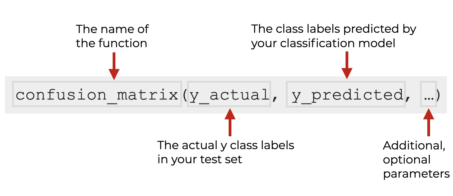
Then, inside the parenthesis, you provide the name of the vector that holds the actual y target labels as the first argument (these are typically the values of the test set).

The second argument is the name of the vector that holds the predicted y labels (also typically from the test data).

The are also a few optional parameters that you can use to modify the behavior of the function.

Let’s quickly look at those.

The Parameters of confusion_matrix

Here, we’ll look the arguments and optional parameters of Scikit Learn confusion_matrix.

• y_actual
• y_pred
• labels
• sample_weight
• normalize

Let’s look at these one at a time.

y_actual (required)

As explained above, the y_actual input should be the vector of actual class labels for every example in your dataset (i.e., the “ground truth” labels).

This should be a Numpy array or array-like object with a shape equal to (n_samples,).

y_pred (required)

The y_predicted input should be the vector of class labels that are predicted by the classifier.

This should also be a Numpy array or array-like object with a shape equal to (n_samples,).

labels

The labels parameter allows you to provide a the names of the class labels.

The argument to this parameter should be a Numpy array or array-like object.

You can provide the full set of class labels, or a subset of labels (in which case, confusion_matrix will operate on that subset of labels).

Importantly, the order that you provide the class labels will dictate the order that the labels appear in the output of confusion matrix. This can be useful for structuring the output of the function in a particular way.

By default, this is set to None, which causes confusion_matrix to use any label that appears in the data.

sample_weight

The sample_weight parameter allows you to set a weight for the different samples (i.e., examples) in the data.

The argument to this parameter should be a Numpy array or array-like object (e.g., a list) of size (n_samples).

By default, this is set to sample_weight = None, which leaves the examples un-weighted.

normalize

The normalize parameter enables a user to get normalized values instead of raw counts.

Effectively, this will provide proportions of the row count, column count, or the total count instead of the raw counts. These proportion values will be in the range between 0 and 1.

Here are the possible arguments to the normalize parameter, and what they do:

• None (default): This removes normalization. In this case, the confusion matrix will contain the absolute counts of correct and incorrect classifications.
• ‘true’: This will apply normalization to every row of the confusion matrix; the rows represent the true labels. Therefore, using normalize = 'true' will divide every row by the sum of that row, and in turn, the sum of each row will be 1. This can give you insight into how the actual classes were predicted by your model, showing the proportion of correct and incorrect predictions for every class.
• ‘pred’: This will apply normalization to every column of the confusion matrix; the columns represent the predicted labels. Therefore, using normalize = 'pred' will divide every column by the sum of that column, and in turn, the sum of each column will be 1. This can help you understand the proportion of true positives, false positives, etc., for every predicted class.
• ‘all’: This applies normalization to the entire matrix. So in this case, every value in the matrix is divided by the total number of observations. This will show the proportion of ever classification outcome with respect to all observations.

Using the normalize parameter can help you better understand a classifier’s performance, particularly when the distribution of classes in the dataset is imbalanced or when you’re more interested in relative performance than raw counts.

The Output of confusion_matrix

For a binary classifier, Sklearn confusion-matrix outputs a matrix where the rows represent the actual classes, and the columns represent the predicted classes.

So it outputs a matrix with true positive, true negative, false positive and false negative are in the following positions:

[[TN, FP],
 [FN, TP]]

Visually, it looks like this:

Although, remember: the above chart shows a confusion matrix that contains the counts of records, but if we use the normalize parameter described above, then instead of counts, we might have proportions instead.

Also note that classification problems with more than 2 class labels, the confusion matrix will be larger than 2×2. For a problem with n classes, the confusion matrix would have size nxn. Having said that, multiclass confusion matrices are more complex, and I’ll write about them more at another time.

Examples of How to Use Sklearn confusion matrix

In this section, I’ll show you how to use the Sklearn confusion matrix function.

Examples:

• Use confusion matrix for binary classification
• Normalize the confusion matrix to get proportions

Run this code first

Before you run the examples, you’ll have to run some setup code first.

Here, we’re going to:

• Make a classification dataset with Sklearn make_classification
• Plot the data with sns.scatterplot
• Split the data with Sklearn train_test_split
• Initialize a Logistic Regression model
• Fit the model with the Sklearn fit method

#--------------------------
# IMPORT PACKAGES AND TOOLS
#--------------------------

import numpy as np
import matplotlib.pyplot as plt
import seaborn as sns
import seaborn.objects as so

from sklearn.datasets import make_classification
from sklearn.model_selection import train_test_split
from sklearn.linear_model import LogisticRegression

from sklearn.metrics import confusion_matrix


# CREATE CLASSIFICAION DATASET
X, y = make_classification(n_samples = 1000
                           ,n_features = 1
                           ,n_informative = 1
                           ,n_redundant = 0
                           ,n_clusters_per_class = 1
                           #,flip_y = 0
                           ,class_sep = 1
                           ,random_state = 2
                           )

X.shape  #(1000,1)
y.shape  #(1000,)


# PLOT DATA
plt.style.use('fivethirtyeight')
plt.figure(figsize = (8,6))
sns.scatterplot(x = X.flatten(), y = y, hue = y)


# CREATE TRAIN & TEST DATA
(X_train, X_test, y_train, y_test) = train_test_split(X, y
                                                      ,test_size = .2
                                                      ,random_state = 22
                                                      )


# INITIALIZE LOGISTIC REGRESSION MODEL
logistic_regressor = LogisticRegression()


# TRAIN MODEL
logistic_regressor.fit(X_train, y_train)

Once you run this, you’ll be ready to run the examples.

EXAMPLE 1: Use confusion matrix for binary classification

Here, we’re going to make a simple confusion matrix for a binary classifier (i.e., the Logistic Regression model that we set up earlier).

Let’s run the code, and then I’ll explain.

from sklearn.metrics import confusion_matrix

# PREDICT Y VALUES
y_pred = logistic_regressor.predict(X_test)

# CREATE AND PRINT CONFUSION MATRIX 
confusion_matrix_data = confusion_matrix(y_test, y_pred)
print(confusion_matrix_data)

OUT:

[[89 14]
 [ 4 93]]

Explanation

Here, we’ve predicted the y values using the Scikit Learn predict method.

Then we took those predicted values, along with the actual y values in y_test, and used them as the inputs to Sklearn confusion_matrix.

The result is the grid of TN, FP, FN, and TP values.

EXAMPLE 2: Normalize the confusion matrix to get proportions

In this example, we’re going to build a confusion matrix that looks a the proportion of the total observations that fall into each quadrant.

To do this, we will set normalize = 'all'.

y_pred = logistic_regressor.predict(X_test)

confusion_matrix_normalized = confusion_matrix(y_test
                                         ,y_pred
                                         ,normalize = 'all'
                                         )
print(confusion_matrix_normalized)

OUT:

[[0.445 0.07 ]
 [0.02  0.465]]

Explanation

By using normalize = 'all', we’ve created a confusion matrix that shows the proportion of total observations that fall into each quadrant.

We could also use other setting for normalize, such as:

• normalize = 'true' to get the row proportions.
• normalize = 'pred' to get the column proportions.

These different variations of the confusion matrix can be used for different perspectives on the performance of a classifier.

Having said that, using and interpreting these different types of confusion matrices can be a big subject, so I’ll write about it more in future blog posts.

Frequently Asked Questions About Scikit-learn confusion matrix

Do you have any unanswered questions about the Scikit-learn confusion matrix function?

Are you still confused about something?

If so, just leave your questions in the comments section at the bottom of the page.

For More Machine Learning Tutorials, Sign Up for our Email List

Confusion matrices are certainly important for machine learning, but if you want to master ML, you’ll have a lot more to learn.

That said, if you want to learn more about machine learning, data science, and AI, then sign up for our email list.

When you sign up, you’ll get free tutorials on:

• NumPy
• Pandas
• Base Python
• Scikit learn
• Machine learning
• Deep learning
• … and more.

If you sign up for the email list, we’ll deliver these free tutorials to you, direct to your inbox.